|
6.2 Reduced-Order State Estimator
In many practical instances, for which only a few states are not measurable, solving the full-order state estimation problem is unnecessary. This problem can be replaced by a reduced-order state estimation problem of finding an  order estimator, where order estimator, where  is the rank of is the rank of  . In the continuous-time case, this amounts to finding the system . In the continuous-time case, this amounts to finding the system


where the matrices  , ,  , ,  , and , and  with dimensions with dimensions  , ,  , ,  , and , and  , respectively, are constructed such that the vector , respectively, are constructed such that the vector  satisfies the system of differential equations Eq. (6.3) and satisfies the system of differential equations Eq. (6.3) and  estimates the states estimates the states  of the original system if the matrix of the original system if the matrix  is stable. Specifically, the error is stable. Specifically, the error  satisfies satisfies
 as as 
where  and and  , , , ,  are eigenvalues of are eigenvalues of  . .
In the discrete-time case, the reduced-order estimator, analogous to the preceding example, is constructed such that the error satisfies
 as as 


Design of the reduced-order state estimator.
ReducedOrderEstimator returns the state-space system with  inputs and inputs and  outputs that can be connected to the original system using the feedback loop shown in Figure 6.1. For outputs that can be connected to the original system using the feedback loop shown in Figure 6.1. For  , the estimator has , the estimator has  states. It is constructed either via the pole assignment approach or the Sylvester-observer equation approach, depending on the value of the option Method. The pole assignment approach, described in Section 6.2.1, is used when the option value is a valid choice for the option Method of the function StateFeedbackGains. Otherwise, the Sylvester-observer equation route, described in Section 6.2.2, is chosen and the option value must be taken from the list given in that section. The default option value corresponds to the pole assignment method and is the default value for StateFeedbackGains. states. It is constructed either via the pole assignment approach or the Sylvester-observer equation approach, depending on the value of the option Method. The pole assignment approach, described in Section 6.2.1, is used when the option value is a valid choice for the option Method of the function StateFeedbackGains. Otherwise, the Sylvester-observer equation route, described in Section 6.2.2, is chosen and the option value must be taken from the list given in that section. The default option value corresponds to the pole assignment method and is the default value for StateFeedbackGains.
For  , ReducedOrderEstimator reconstructs the state variables as , ReducedOrderEstimator reconstructs the state variables as  , where , where  and and  is the pseudoinverse of the matrix is the pseudoinverse of the matrix  . In that case, ReducedOrderEstimator returns a state-space system with only the direct transmission term. . In that case, ReducedOrderEstimator returns a state-space system with only the direct transmission term.
Make sure that the package is available.
In[1]:=
Load the collection of test examples.
In[2]:=
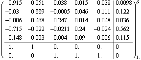
This is a model of a steam power system.
In[3]:=
Out[3]=
This selects the estimator poles.
In[4]:=
Out[4]=
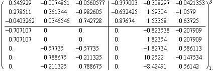
This finds the reduced-order state estimator with  states, states,  inputs, and inputs, and  outputs. outputs.
In[5]:=
Out[5]=
Here are the initial values for the randomly selected states.
In[6]:=
This selects the length of the input signal and output measurements.
In[7]:=
This prepares a sinusoidal input signal.
In[8]:=
This is the output response to the sinusoidal input signal.
In[9]:=
The estimated state response is obtained by feeding the true input and output to the reduced-order state estimator.
In[10]:=
This is the true state response.
In[11]:=
This loads the standard package.
In[12]:=
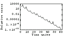
This graphs the relative error of the estimated states with respect to the simulated true states.
In[13]:=

The graph clearly shows that the error decays exponentially. The slope of the line is governed by the "most unstable" pole of the estimator, which in this particular case is given by  . .
|