|
2. Introduction: Extending Mathematica to Solve Control Problems
In this chapter, using the classical example of controlling an inverted pendulum, we learn how to formulate a control problem in Mathematica, solve the problem using the Control System Professional functionality, and analyze the results using the standard Mathematica functions. We will see that, by being seamlessly incorporated with the rest of Mathematica, this application package provides a convenient environment for solving typical control engineering problems. Additional solved examples will be given in later chapters when individual functions are discussed.
The inverted pendulum shown in Figure 2.1 is a massive rod mounted on a cart that moves in a horizontal direction in such a way that the rod remains vertical. The vertical position of the rod is unstable, and the cart exerts a force to provide the attitude control of the pendulum. This or a similar model is considered in many textbooks on control systems. We will follow Brogan (1991), pp. 590-92.
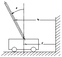
Figure 2.1. Inverted pendulum.
Let us obtain a mathematical model for the system. Assume that the length of the pendulum is  , and its mass and the moment of inertia about its center of gravity are , and its mass and the moment of inertia about its center of gravity are  and and  , respectively. The mass of the cart is , respectively. The mass of the cart is  . Then, summing the forces applied to the pendulum in horizontal and vertical directions (Figure 2.2a), we have . Then, summing the forces applied to the pendulum in horizontal and vertical directions (Figure 2.2a), we have
  where  and and  are the components of the reaction force at the support point, and are the components of the reaction force at the support point, and  and and  are the horizontal and vertical displacements of the center of gravity of the pendulum; are the horizontal and vertical displacements of the center of gravity of the pendulum;  depends on the horizontal displacement depends on the horizontal displacement  of the cart. Summing all the moments around the center of gravity of the pendulum gives the dynamical equation of the cart. Summing all the moments around the center of gravity of the pendulum gives the dynamical equation
 where  , which corresponds to the case of uniform mass distribution along the pendulum. , which corresponds to the case of uniform mass distribution along the pendulum.
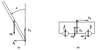
Figure 2.2. Forces applied to the rod (a) and the cart (b) of the pendulum.
Finally, for the cart we have (see Figure 2.2b)
 where  is the input force applied to the wheels. is the input force applied to the wheels.
Translating the model into Mathematica is straightforward.
This is the first equation. We will keep it as eq1 for future reference.
In[1]:=
Out[1]=
The next equation translates almost verbatim as well.
In[2]:=
Out[2]=
This is the dynamical equation.
In[3]:=
Out[3]=
This gives the definition for the moment of inertia J.
In[4]:=
Out[4]=
Here is the last equation.
In[5]:=
Out[5]=
We now define the horizontal displacement xc of the pendulum through the displacement of the cart X and the angle  . As the two depend on time t, then so does xc. The pattern notation t_ on the left-hand side makes the formula work for any expression t. . As the two depend on time t, then so does xc. The pattern notation t_ on the left-hand side makes the formula work for any expression t.
In[6]:=
Out[6]=
Here is the corresponding assignment to the vertical displacement yc.
In[7]:=
Out[7]=
Notice that we have defined eq1  eq4 as logical equations (using the double equation mark ==) and the expressions for xc and yc as assignments to these symbols (using the single =). We then have the benefit of not solving the differential equation against eq4 as logical equations (using the double equation mark ==) and the expressions for xc and yc as assignments to these symbols (using the single =). We then have the benefit of not solving the differential equation against  , but simply eliminating it algebraically along with the other variables we no longer need. , but simply eliminating it algebraically along with the other variables we no longer need.
Eliminate takes the list of equations and the list of variables to eliminate. The result is a nonlinear differential equation between the input force fx and the angular displacement  and its first and second derivatives. It is solvable for and its first and second derivatives. It is solvable for  . .
In[8]:=
Out[8]=
Solve returns a list of rules that give generic solutions to the input equation.
In[9]:=
Out[9]=
We have, in fact, just a single rule and we extract it from the lists.
In[10]:=
Out[10]=
As our next step, we create a state-space model of the system and linearize it for small perturbations near the equilibrium position  . Then, based on the linearized model, we design the state feedback controller that attempts to keep the pendulum in equilibrium. Finally, we carry out several simulations of the actual nonlinear system governed by the controller and see what such a controller can and cannot do. . Then, based on the linearized model, we design the state feedback controller that attempts to keep the pendulum in equilibrium. Finally, we carry out several simulations of the actual nonlinear system governed by the controller and see what such a controller can and cannot do.
The nonlinear state-space model of the system will be presented in the form
 where  and and  constitute the state vector constitute the state vector  , ,  is the only component of the input vector is the only component of the input vector  , and , and  makes up the output vector makes up the output vector  . .
This creates the state vector in Mathematica.
In[11]:=
This sets the input and output vectors.
In[12]:=
To obtain  and and  in Eq. (2.5), we observe that their Mathematica equivalents f and h are simply the derivative D[x, t] and the output vector y expressed via the state and input variables. in Eq. (2.5), we observe that their Mathematica equivalents f and h are simply the derivative D[x, t] and the output vector y expressed via the state and input variables.
The expression for the derivative contains an undesirable variable,  , which is among neither state nor input variables. , which is among neither state nor input variables.
In[13]:=
Out[13]=
The replacement rule stored as sln helps to get rid of  . .
In[14]:=
Out[14]=
The expression for function h is trivial.
In[15]:=
Out[15]=
So far we have used the built-in Mathematica functions. Now it's time to make accessible the library of functions provided in Control System Professional.
This loads the application.
In[16]:=
For most Control System Professional functions, the input state-space model must be linear. Therefore, our first task will be to linearize the model, that is, represent it in the form
 This is the purpose of the function Linearize, which, given the nonlinear functions f and h and the lists of state and input variables, supplied together with values at the nominal point (the point in the vicinity of which the linearization will take place), returns the control object StateSpace[a, b, c, d], where matrices a, b, c, and d are the coefficients  , ,  , ,  , and , and  in Eq. (2.6). in Eq. (2.6).
This performs the linearization.
In[17]:=
Out[17]=
Mapping the built-in Mathematica function Factor onto components of the state-space object simplifies the result somewhat. (Here /@ is a shortcut for the Map command.)
In[18]:=
Out[18]=
TraditionalForm often gives a more compact representation for control objects.
In[19]:=
Out[19]//TraditionalForm=
Now let us design a state feedback controller that will stabilize the pendulum in a vertical position near the nominal point. One way to do this is to place the poles of the closed-loop system at some points  and and  on the left-hand side of the complex plane. on the left-hand side of the complex plane.
In this particular case, Ackermann's formula (see Section 9.1) is used. The result is a matrix comprising the feedback gains.
In[20]:=
Out[20]=
Note that we were able to obtain a symbolic solution to this problem and thus see immediately that, for example, only the first gain depends on  and so would be affected should our pendulum get sent to Mars (and the change would be linear in and so would be affected should our pendulum get sent to Mars (and the change would be linear in  ). We also see that the first gain depends on the product of pole values, the second gain on their sum, and so on. ). We also see that the first gain depends on the product of pole values, the second gain on their sum, and so on.
To check if the pole assignment has been performed correctly, we can find the poles of the closed-loop system, that is, the eigenvalues of the matrix  . .
This extracts the matrices from their StateSpace wrapper.
In[21]:=
We see that the eigenvalues of the closed-loop system are indeed as required.
In[22]:=
Out[22]=
With Control System Professional, we can also design the state feedback using the optimal linear-quadratic (LQ) regulator (see Chapter 10). This approach is more computationally intensive, so it is advisable to work with inexact numeric input. For convenience in presenting results, we switch to the control print display (Section 1.5).
This is the particular set of numeric values (all in SI) we will use.
In[23]:=
Out[23]=
Here our system is numericalized.
In[24]:=
Out[24]=
Let  and and  be identity matrices. be identity matrices.
In[25]:=
Out[25]=
In[26]:=
Out[26]=
LQRegulatorGains solves the Riccati equations and returns the corresponding gain matrix.
In[27]:=
Out[27]=
Here are the poles our system will possess when we close the loop.
In[28]:=
Out[28]=
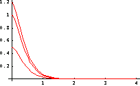
Let us make some simulations of the linearized system as well as the original, nonlinear system stabilized with one of the controllers we have designed—say the one obtained with Ackermann's formula. We start with the linearized system and compute the transient response of the system for the initial values of  of 0.5, 1, and 1.2, assuming in all cases that of 0.5, 1, and 1.2, assuming in all cases that  . The same initial conditions will then be used for the nonlinear system, and the results will be compared. . The same initial conditions will then be used for the nonlinear system, and the results will be compared.
Here is the list of initial conditions for  . .
In[29]:=
Out[29]=
This is the linearized system after the closing state feedback. The function StateFeedbackConnect is described in Chapter 6 together with other utilities for interconnecting systems.
In[30]:=
Out[30]=
To compute how the initial condition in  decays in the absence of an input signal, we can use OutputResponse, which is one of the functions defined in Chapter 4. decays in the absence of an input signal, we can use OutputResponse, which is one of the functions defined in Chapter 4.
In this particular case, the input arguments to OutputResponse are the system to be analyzed, the input signal (which is 0 for all t), the time variable t, and the initial conditions for the state variables supplied as an option. The initial value for  is denoted as angle. is denoted as angle.
In[31]:=
Out[31]=
Here is the plot of the previous function for the chosen values . We store it as plot for future reference.
In[32]:=
The case of actual nonlinear system stabilized with the linear controller is more interesting, but requires some work on our part. We note that when the control loop is closed, the input variable—the force  applied by the motor of the cart—tracks changes in state variables applied by the motor of the cart—tracks changes in state variables  and and  . .
First we prepare the input rules. As we have only one input, there is only one rule in the list.
In[33]:=
Out[33]=
Recall that we store the description of our nonlinear system as sln.
In[34]:=
Out[34]=
Now we numericalize the rule, substitute the feedback rules, and, to convert the rule to an equation, apply the head Equal to it (@@ is the shorthand form of the Apply function). The resultant differential equation is labeled de.
In[35]:=
Out[35]=
This solves the differential equation with the initial conditions for every value in the list one by one and returns a list of solutions. The time t is assumed to vary from 0 to 4 seconds.
In[36]:=
Out[36]=
In several graphs that follow, we show the results for  as a solid line, for as a solid line, for  as a dashed-dotted one, and for as a dashed-dotted one, and for  as a dashed line. This changes the Plot options to reflect that convention and adjusts a few other nonautomatic values for plot options. as a dashed line. This changes the Plot options to reflect that convention and adjusts a few other nonautomatic values for plot options.
In[37]:=
The results for  are now presented graphically. We can see that the controller succeeds in driving the pendulum to its equilibrium position for all three initial displacements. The plot is stored as plot1. are now presented graphically. We can see that the controller succeeds in driving the pendulum to its equilibrium position for all three initial displacements. The plot is stored as plot1.
In[38]:=
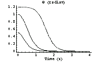
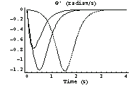
We can also see that, once the angle  [t] has come to zero, the derivative [t] has come to zero, the derivative  vanishes as well. This means that the pendulum is not about to oscillate around its equilibrium position, at least not when driven from the displacements we are considering for now. vanishes as well. This means that the pendulum is not about to oscillate around its equilibrium position, at least not when driven from the displacements we are considering for now.
In[39]:=
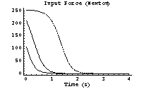
Here is the plot of input force versus time.
In[40]:=
Finally, we compare the graphs of  for the nonlinear and linear systems and see that the only case of smallest initial displacement is treated adequately by the linear model. for the nonlinear and linear systems and see that the only case of smallest initial displacement is treated adequately by the linear model.
In[41]:=
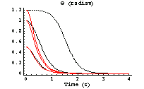
The transient responses suggest that our linear feedback is not sufficiently prompt in reacting to moderate and large initial displacements  , and that may cause problems for still larger angles. The case , and that may cause problems for still larger angles. The case  rad is almost critical. Indeed, for a slightly larger displacement, rad is almost critical. Indeed, for a slightly larger displacement,  rad, the system becomes hard to control. rad, the system becomes hard to control.
We solve the same equation for another set of initial conditions.
In[42]:=
Out[42]=
In the following graphs, we will plot the results for  as a solid line and one of our previous curves (namely, as a solid line and one of our previous curves (namely,  ) as a dashed line. This sets the new options. ) as a dashed line. This sets the new options.
In[43]:=
We find that the pendulum still could be driven from  to to  , but now it oscillates badly around the equilibrium point. , but now it oscillates badly around the equilibrium point.
In[44]:=
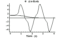
Of course, the cart in our particular model of the pendulum (as shown in Figure 2.1) would not allow the pendulum to rotate in circles, but, for the sake of argument, we will assume that it would.
The variations in  become more complex and far more intense. become more complex and far more intense.
In[45]:=
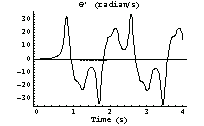
This is the force the motor must exert to maintain the process.
In[46]:=
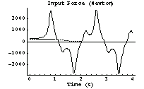
The real actuator may not be up to the task. If the maximum force the motor can provide is, say,  N, and the feedback saturates at that limit, the controller fails to balance the pendulum. N, and the feedback saturates at that limit, the controller fails to balance the pendulum.
To model this situation, we create a clip function.
In[47]:=
Out[47]=
Here is how it works: everything beyond the interval from  to to  gets cut off. gets cut off.
In[48]:=
Out[48]=
We use clip to saturate the feedback.
In[49]:=
Out[49]=
This is the new differential equation for  under the saturated feedback. under the saturated feedback.
In[50]:=
Out[50]=
This solves it.
In[51]:=
Out[51]=
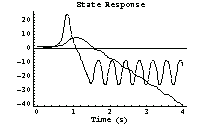
Finally, we plot the state response—for  as a solid line and for as a solid line and for  as a dashed one. It is clear that the controller fails to return the pendulum to its equilibrium position. as a dashed one. It is clear that the controller fails to return the pendulum to its equilibrium position.
In[52]:=
|