|
5.2 The Bode Plot
5.2.1 The Basic Function
The Bode plot is the first example of the frequency response analysis tools that we consider in this chapter. By frequency response, we mean the response to purely sinusoidal signals. BodePlot depicts, in the form of GraphicsArray, the frequency dependence of the magnitude and phase response. The magnitude response is the ratio of the span of the output sinusoid to the input one, and the phase response is the phase difference between them. The magnitude and phase dependencies are plotted in the double-logarithmic and semilogarithmic scales, respectively.


Creating the Bode plots.
Like all other plotting routines in Control System Professional, BodePlot accepts a system in state-space or transfer function form in the continuous- or discrete-time domain. Specifying the frequency range is optional. If it is not supplied, BodePlot will try to determine a suitable range automatically. Also optional is the naming of the frequency variable in supplying the desired frequency range; {w, wmin, wmax works as well as {wmin, wmax works as well as {wmin, wmax . This should come as no surprise if you recall that the variable in TransferFunction is an internal parameter and does not have any meaning outside the scope of the TransferFunction object. . This should come as no surprise if you recall that the variable in TransferFunction is an internal parameter and does not have any meaning outside the scope of the TransferFunction object.
Consider again the second-order system.
In[11]:=
This is the Bode plot for the unity natural frequency and damping ratio. The frequency range is not specified and is determined automatically.
In[12]:=
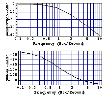
This gives the Bode plot over a wider frequency range.
In[13]:=
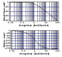
By default, BodePlot tries to unwrap the phase in order to present a smooth phase curve should branch cuts be detected. The value Automatic for the option PhaseRange typically (unless the gain and phase margins are to be plotted—see below) corresponds to such behavior. PhaseRange allows also to shift the graph to another phase range which must be specified in the form PhaseRange {min, max {min, max , with the new limits min and max given in degrees. Very rapid changes in phase dependence may cause errors in phase unwrapping. The safest (and fastest) choice is PhaseRange , with the new limits min and max given in degrees. Very rapid changes in phase dependence may cause errors in phase unwrapping. The safest (and fastest) choice is PhaseRange  {-180, 180}, in which case no additional processing of the phase is performed. {-180, 180}, in which case no additional processing of the phase is performed.
Another way to eliminate possible errors in phase unwrapping is to increase the number of points at which the transfer function is sampled by changing the option PlotPoints; this is also useful if rapid changes in the magnitude or phase curve are not plotted satisfactorily otherwise. For some plots, you may wish to use linear spacing between samples instead of the default logarithmic spacing. This can be done by using PlotSampling  LinearSpacing. LinearSpacing.
The option PhaseRange is in no way a substitute for the standard Mathematica plotting option PlotRange and, in fact, works quite differently. If, for example, a plot does not have any part in the range specified in PlotRange, nothing will appear in the graph. On the other hand, PhaseRange will bring the graph into the specified range based on the principle that all  intervals are physically equivalent. intervals are physically equivalent.
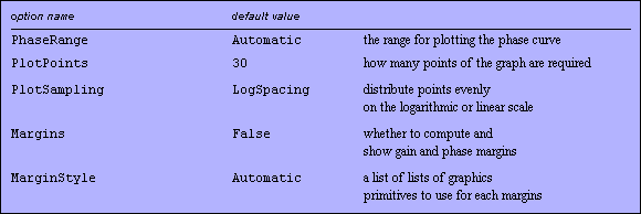
Options specific to BodePlot.
BodePlot also accepts options pertinent to ListPlot and GraphicsArray. Because a plot consists of two subplots, certain options—namely, AspectRatio, AxesLabel, AxesOrigin, FrameLabel, Epilog, Prolog, FrameTicks, GridLines, Ticks, and PlotRange—are handled in a nonstandard fashion. Given a list of two items as input, they will apply the first item to the magnitude plot and the second to the phase plot. Other options are applied equally to both plots or to GraphicsArray itself.
BodePlot operates on MIMO systems by grouping the graphs related to each input and plotting as many graphs as there are inputs. You may specify options for each input differently by wrapping option values into additional list. By default, the graphs related to different outputs in one plot are distinguished by the Hue value. This can be changed using the standard PlotStyle option.
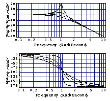
Here is a single-input, multiple-output system, of which each input-output pair is a second-order system with a different value of damping ratio.
In[14]:=
Out[14]=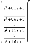
This is its Bode plot.
In[15]:=
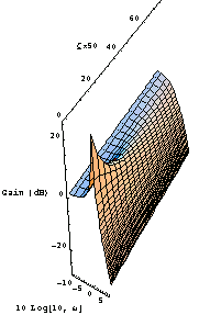
Of course, you can always supplement the results from BodePlot with diagrams obtained using the built-in Mathematica functions. This plots the gain versus frequency and damping ratio for the generic second-order system. To make a more attractive graphic, we picked up some coefficients for the  and and  axes. axes.
In[16]:=
|