9.1 Pole Assignment with State Feedback

By closing the loop of an -order system

with the state feedback control , one forces the system's poles, that is, the eigenvalues of matrix , to assume the new positions

The problem of finding the matrix that yields the desired locations of poles is often referred to as the pole assignment or pole placement problem. The function StateFeedbackGains attempts to find its solution, assuming that the input system is completely controllable. So long as the algorithm does not require knowledge of matrices and , they may be omitted in the state-space description of the input system.

State feedback design.

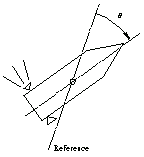
As an example, we consider a model of the single-axis satellite control system depicted in Figure 9.1. The transfer function for the system is , where is the angle of the satellite axis with respect to a reference, is the normalized input variable,  is the control torque applied by the thruster, and  is the moment of inertia about the center of mass (Franklin et al. (1990)).

Figure 9.1. One-degree-of-freedom model of satellite attitude control.

Load the application.

In[1]:=<<ControlSystems`

This is the transfer function for the satellite control system.

In[2]:=

Out[2]=

This finds a discrete-time realization of the system for sampling period .

In[3]:=

Out[3]=

This designs the discrete-time controller that would place the poles of this system into the desired locations and in the complex plane.

In[4]:=

Out[4]=

This is the controller gain matrix for the particular case and sampling period seconds.

In[5]:=

Out[5]=

Feedback design is prone to significant numerical errors, especially for high-order or weakly controllable systems. StateFeedbackGains has several options that help to avoid meaningless results. There are also some options pertaining to the method being applied.

Some of the options for StateFeedbackGains.

The option Method determines what method to use to compute the feedback gains. In the base package, two methods are available: Ackermann and KNVD. The option value Automatic imposes the following division of labor: KNVD is called for inexact input and for a special case of exact input, namely, when the number of inputs is equal to the number of states; Ackermann is used otherwise.

Using the option VerifyPoles, it is possible to check if the poles of the closed-loop system are indeed (close to) the required ones. For the option value Automatic, the check is made only if the input is inexact. The value must be set to True to perform the check on exact input or input containing symbolic expressions. The option can be set to False to save some computing time.

The option AdmissibleError relates to the option VerifyPoles and specifies the relative error in the location of poles that is deemed admissible. The value in no way affects the result of the computation. If the required accuracy has not been reached, it is up to the user to choose the appropriate strategy. Traditionally, the case would require changing the method of computation, reconsidering the requirement for accuracy, or even reformulating the problem. In Mathematica, one may also use a built-in mechanism for manipulating the precision, which may resolve some problems of this sort.

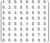
Consider a hypothetical eighth-order system.

In[6]:=

In[7]:=

Out[7]=

In[8]:=

Out[8]=

Suppose this is the list of the desired pole locations after the loop is closed.

In[9]:=

Out[9]=

Let us try to place the poles using Ackermann's formula (defined shortly) while making sure that the target is not missed by more than percent. We are warned that the goal has not been achieved. (Since we are not particularly interested in the concrete values of the gains, we suppress the output by placing the semicolon in the end of the input statement.)

In[10]:=

On our machine, the machine-precision numbers are 16 digits long.

In[11]:=

Out[11]=

This increases the precision of our parameters.

In[12]:=

By increasing the precision of the input, we force the feedback computation to be done with higher precision. Now we are presented with no warning.

In[13]:=

We double-check the result. The achieved accuracy is even greater than required.

In[14]:=

Out[14]=