|
9.2 State Reconstruction
The prerequisite for pole assignment using state feedback is knowledge of the state variables. So far in this chapter we have assumed that this prerequisite was somehow met. Now we address the problem of how that can be done. In the trivial case of a square nonsingular matrix  , the state vector can simply be computed from the input and output vectors as , the state vector can simply be computed from the input and output vectors as  ; otherwise an attempt can be made to reconstruct the state vector by forming a device called an estimator (or observer), with which the approximation ; otherwise an attempt can be made to reconstruct the state vector by forming a device called an estimator (or observer), with which the approximation  to the state vector to the state vector  can be obtained as can be obtained as
 where  is the estimator gain matrix. Figure 9.4 presents such a device in block diagram form (Brogan (1991)). As seen from the diagram, that the estimator is driven by the difference between the actual output measurement is the estimator gain matrix. Figure 9.4 presents such a device in block diagram form (Brogan (1991)). As seen from the diagram, that the estimator is driven by the difference between the actual output measurement  and the "expected" output and the "expected" output  , provided that the direct transmission term , provided that the direct transmission term  is taken into account. is taken into account.
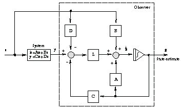
Figure 9.4. Continuous-time estimator schematic.
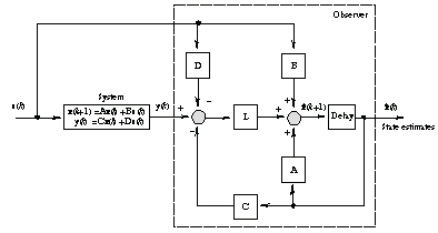
Figure 9.5. Discrete-time estimator schematic.
If the initial system is completely observable, it is possible to choose gains  to be such that the eigenvalues of to be such that the eigenvalues of  assume any desired location, thereby controlling the rate at which assume any desired location, thereby controlling the rate at which  follows follows  . This reduces the problem of finding the estimator gains to one of finding the (transposed) controller gains for the dual system: . This reduces the problem of finding the estimator gains to one of finding the (transposed) controller gains for the dual system:
 Therefore, the function StateFeedbackGains can be employed for the purpose. Alternatively, one may use the function EstimatorGains, which performs the procedure in one step. EstimatorGains does not introduce any new options of its own, but accepts and passes on the options for StateFeedbackGains and DualSystem.


Estimator design.
The preceding diagram and equations refer to continuous-time systems. The estimator for a discrete-time system is determined by an equation similar to Eq. (9.4):
 the corresponding block diagram is presented in Figure 9.5. EstimatorGains handles both continuous- and discrete-time cases.
Another linearized state-space model of an inverted pendulum, reproduced after Gopal (1993), will be used in the rest of this section to illustrate obtaining the estimator gain matrix. The model assumes that the state and input vectors are, respectively,
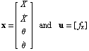
where  is the angular displacement of the pendulum, is the angular displacement of the pendulum,  is the horizontal position of the cart, and is the horizontal position of the cart, and  is the external force applied to the wheels. The model further assumes that the only variable available for measurement is is the external force applied to the wheels. The model further assumes that the only variable available for measurement is  , making it, therefore, the only output variable: , making it, therefore, the only output variable:

Here is the state-space model.
In[27]:=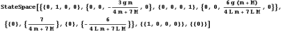
Out[27]=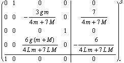
Because we know that all symbolic variables in the input system are real-valued, we may set the option ComplexVariables correspondingly to get a simpler result. This option will be picked up by the function DualSystem. At this point, we will not specify the desired poles for the estimator, but use a generic list of four symbolic values, {p1, p2, p3, p4}. Therefore, the expression will be obtained in its general form.
This finds the estimator for the system and somewhat simplifies the result.
In[28]:=
Out[28]=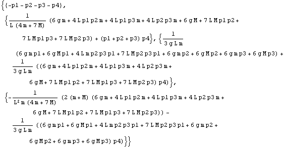
This is the result for a particular set of numerical values.
In[29]:=
Out[29]=
|