|
12.2 Lyapunov Equations
The function LyapunovSolve attempts to find the solution  to the Lyapunov equation to the Lyapunov equation
 a special class of linear matrix equations that occurs in many branches of control theory, such as stability analysis, optimal control, and response of a linear system to white noise (see, e.g., Brogan (1991)). Typically,  and and  are square matrices with dimensions are square matrices with dimensions  and and  . To be consistent, matrices . To be consistent, matrices  and and  should have dimensions should have dimensions  . An important particular case of the Lyapunov equation, . An important particular case of the Lyapunov equation,
 involves only matrices  and and  , in which case all matrices are square with the same dimensions. , in which case all matrices are square with the same dimensions.
For discrete-time systems, the discrete Lyapunov equation,
 arises. The solution can be found with DiscreteLyapunovSolve.


Functions for solving Lyapunov equations.
Here is some matrix a.
In[12]:=
Here is matrix c.
In[13]:=
This solves the discrete Lyapunov equation and simplifies the result.
In[14]:=
Out[14]=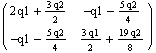
We may verify that the solution indeed satisfies the discrete Lyapunov equation.
In[15]:=
Out[15]=
Consider now an example of design of a feedback controller that uses Lyapunov's method to approximate the minimum-time response system for a given system (see Brogan (1991), Section 10.8). The method is applicable to systems stable at least in Lyapunov's sense. To find the Lyapunov function   , we will first solve the Lyapunov equation, , we will first solve the Lyapunov equation,  , where , where  is the identity matrix with proper dimensions. Knowing is the identity matrix with proper dimensions. Knowing  , one can find , one can find    . To make . To make  as negative as possible, and thereby obtain the fastest response, we will compute the input signal as as negative as possible, and thereby obtain the fastest response, we will compute the input signal as

These are matrices  and and  for a state-space system, which we assume to be continuous-time. for a state-space system, which we assume to be continuous-time.
In[16]:=
In[17]:=
This solves the Lyapunov equation. The matrix  is assumed to be the identity matrix is assumed to be the identity matrix  . .
In[18]:=
Out[18]=
This computes the control law.
In[19]:=
In[20]:=
Out[20]=
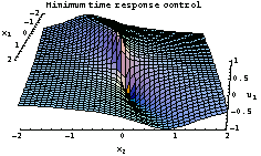
Despite the fact that our system is linear, the minimum time response control is not.
This plot shows the first control signal as a function of the state variables.
In[21]:=
This is the second component of the control signal.
In[22]:=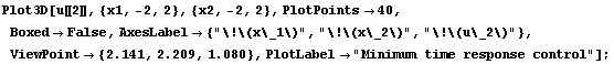
LyapunovSolve and DiscreteLyapunovSolve use the direct method (via the built-in function Solve) or the eigenvalue decomposition method. The method is set using the option SolveMethod, which correspondingly accepts the values DirectSolve and Eigendecomposition. If this option's value is Automatic, these methods are tried in turn until one succeeds or all are tried.

Option specific to Lyapunov equation solvers.
|