|
11.1 Local Linearization of Nonlinear Systems
For a nonlinear state-space system of the form
 the locally linearized model is given by
 where  , ,  , and , and  are small deviations, are small deviations,

from some known solution  , ,  , and , and  to the original nonlinear Eq. (11.1), which we refer to as the nominal solution. The coefficients to the original nonlinear Eq. (11.1), which we refer to as the nominal solution. The coefficients  , ,  , ,  , and , and  are the Jacobian matrices evaluated on the nominal solution: are the Jacobian matrices evaluated on the nominal solution:
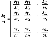
 where the Jacobian  for a vector of functions for a vector of functions
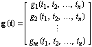
in variables  is is
The function Linearize attempts to find such an approximation.


Local linearization.
Linearize accepts one or both of the function vectors  and and  and returns, respectively, the short (containing just matrices and returns, respectively, the short (containing just matrices  and and  ) or full (containing all four matrices) state-space description. Desired options for the resulting state-space object may be supplied to Linearize or inserted later. ) or full (containing all four matrices) state-space description. Desired options for the resulting state-space object may be supplied to Linearize or inserted later.
As an example, we consider the linearization of the one-dimensional magnetic ball suspension system shown in Figure 11.1 (after Kuo (1991)). The system attempts to control the vertical position  of the steel ball through input voltage of the steel ball through input voltage  . The state variables are chosen as . The state variables are chosen as  , ,  , and , and  . The only input variable is . The only input variable is  . .
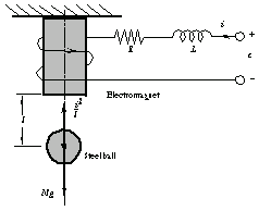
Figure 11.1. Magnetic ball levitation system.
Load the application.
In[1]:=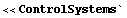
This is vector  corresponding to the nonlinear state equation corresponding to the nonlinear state equation  . .
In[2]:=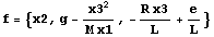
Out[2]=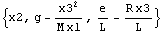
The output vector contains a single variable. Linearize does not require additional list wrapping in such a case.
In[3]:=
Out[3]=
This linearizes the state equation near some nominal point with the coordinates x10, x20, x30, and e0. Since only one vector (f) is supplied, the resulting state-space object contains only two matrices,  and and  . .
In[4]:=
Out[4]=
This finds the full (four-matrix) state-space description.
In[5]:=
Out[5]=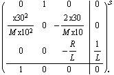
As soon as the linearized state-space model is found, we may apply other Control System Professional functions. For this experiment, let the nominal point be the equilibrium position of the ball at some coordinate l0.
In[6]:=
Out[6]=
This is the state-space description near the equilibrium.
In[7]:=
Out[7]=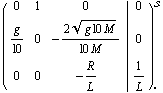
We now find the state feedback gain matrix that places the poles of the system into some position p1, p2, p3.
In[8]:=
Out[8]=
This is the system after the feedback loop is closed.
In[9]:=
Out[9]=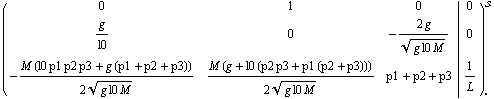
This is the closed-loop system for a particular set of numerical parameters after dropping insignificant numerical errors.
In[10]:=
Out[10]=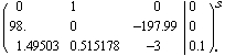
Let us investigate the dynamics of the state variables. One way to do this is to insert an identity matrix as matrix  into the previous (short) state-space object to feed all states through to the outputs. The matrix can be directly inserted at the last position in the state-space object. into the previous (short) state-space object to feed all states through to the outputs. The matrix can be directly inserted at the last position in the state-space object.
In[11]:=
Out[11]//StandardForm=
In[12]:=
Out[12]=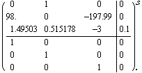
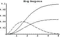
This gives the state response to a step function, that is, it shows how the state variables change if the input voltage applied to the electromagnet suddenly changes by some value ( mV in the plot). The coordinate and velocity of the ball are shown as a solid and dashed line, respectively, and the current in the magnet is shown as the dashed-dotted line. mV in the plot). The coordinate and velocity of the ball are shown as a solid and dashed line, respectively, and the current in the magnet is shown as the dashed-dotted line.
In[13]:=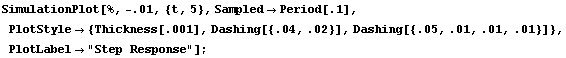
|