|
10.3 Riccati Equations
Finding the optimal control for a continuous-time linear system with a quadratic cost function involves solving the differential Riccati equation, which, for the case of infinite-horizon problem, simplifies to the algebraic Riccati equation (ARE)
 The discrete-time case requires solution of the discrete algebraic Riccati equation (DARE)
 (see, for example, Brogan (1991), Section 14). These are equations in an unknown matrix  that could be viewed as systems of coupled quadratic equations regarding the unknown components that could be viewed as systems of coupled quadratic equations regarding the unknown components  and as such could be attempted using the built-in Mathematica functions Solve and NSolve. Control System Professional provides also two more specialized functions that can be more efficient than the general-purpose solvers. and as such could be attempted using the built-in Mathematica functions Solve and NSolve. Control System Professional provides also two more specialized functions that can be more efficient than the general-purpose solvers.


Functions for solving Riccati equations.
Consider again the double-integrator system.
In[20]:=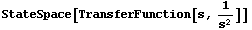
Out[20]=
This extracts matrices  and and  . .
In[21]:=
Let all the weights be equal.
In[22]:=
This is the solution to the corresponding ARE.
In[23]:=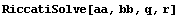
Out[23]=
Consider now another second-order system.
In[24]:=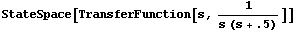
Out[24]=
This time we find its discrete-time equivalent for a sampling period of, say,  second. second.
In[25]:=
Out[25]=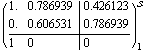
This extracts matrices  and and  . .
In[26]:=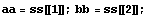
This solves the DARE.
In[27]:=
Out[27]=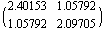
We can use the result to find the optimal feedback gains.
In[28]:=
Out[28]=
We could also arrive at this result by using LQRegulatorGains directly.
In[29]:=
Out[29]=
For yet another example, let us design a controller for the roll attitude of a missile (Figure 10.2). The controller must, by using the hydraulic-powered ailerons, keep roll attitude  close to zero while staying within the physical limits of aileron deflection close to zero while staying within the physical limits of aileron deflection  and aileron deflection rate and aileron deflection rate  (Bryson and Ho (1969)). In the state-space description, it is assumed that the system has one input, which accepts the command signal to aileron actuators (Bryson and Ho (1969)). In the state-space description, it is assumed that the system has one input, which accepts the command signal to aileron actuators  so that so that  and the state vector is and the state vector is

The performance index we choose is
resulting in matrices  and and  as shown below. as shown below.  and and  are the maximum desired values of are the maximum desired values of  and and  , and , and  is the maximum available value of is the maximum available value of  . .
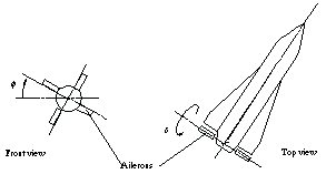
Figure 10.2. Roll attitude control of a missile.
This is the  matrix for the model. Q and matrix for the model. Q and  are the aileron effectiveness and roll-time constant, respectively. are the aileron effectiveness and roll-time constant, respectively.
In[30]:=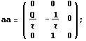
This is matrix  . .
In[31]:=
These are the matrices  and and  for the performance index. for the performance index.
In[32]:=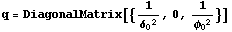
Out[32]=
In[33]:=
Out[33]=
We choose a set of numeric values for our parameters.
In[34]:=
Out[34]=
We then reassign the matrices using these values.
In[35]:=
Applying RiccatiSolve to this list solves the corresponding Riccati equation.
In[36]:=
Out[36]=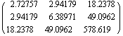
We can use the solution to find the optimal feedback matrix.
In[37]:=
Out[37]=
Again, the result is the same as the one obtained with LQRegulatorGains.
In[38]:=
Out[38]=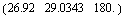
RiccatiSolve and DiscreteRiccatiSolve work by finding the eigensystem of the corresponding Hamiltonian matrix. Alternatively, one may use the Schur decomposition method, which has advantages for systems with multiple or near-multiple eigenvalues of the Hamiltonian (Laub (1979)). The method is accessible by selecting the option SolveMethod  SchurDecomposition (which is available for RiccatiSolve only). If this method is chosen, RiccatiSolve does not accept infinite-precision input since neither does the built-in function SchurDecomposition. The default Automatic setting of the option selects the Eigendecomposition or SchurDecomposition method depending on whether the input matrices are exact or not (for DiscreteRiccatiSolve, Eigendecomposition is chosen in either case). SchurDecomposition (which is available for RiccatiSolve only). If this method is chosen, RiccatiSolve does not accept infinite-precision input since neither does the built-in function SchurDecomposition. The default Automatic setting of the option selects the Eigendecomposition or SchurDecomposition method depending on whether the input matrices are exact or not (for DiscreteRiccatiSolve, Eigendecomposition is chosen in either case).

Option specific to RiccatiSolve.
Solving Riccati equations involves sorting eigenvalues of the Hamiltonian (which is required to separate stable and unstable eigenvalues); therefore, the eigenvalues should not contain symbolic parameters. If symbolic parameters are used, a warning is issued and LQRegulatorGains returns unevaluated. This, of course, does not mean that the system cannot be solved symbolically; however, such a case requires human intervention in the selection of stable poles.
|