|
10.5 Optimal Estimation
Section 9.2 introduced the device called the estimator (or observer) and the function EstimatorGains, which computes the gain matrix for the device. Input and output measurements were assumed to be known precisely so the problem could be referred to as the deterministic state reconstruction. Consider now a linear system whose state vector is subject to some random disturbances  , called the process noise, and whose output measurements are contaminated with noise , called the process noise, and whose output measurements are contaminated with noise  , called the measurement noise , called the measurement noise
 The noise processes are assumed to have flat spectra (white noise), zero mean values

and covariance matrices  and and 

Here  denotes the mean of random variable denotes the mean of random variable  . The two noises may further be assumed to be mutually uncorrelated, . The two noises may further be assumed to be mutually uncorrelated,

or if they are correlated, then their cross-covariance matrix is  : :

If the observer with the same structure as in Figure 9.4 (Figure 9.5 for the discrete-time case) is applied to find the state estimates from noisy measurements, and the dual algorithm to the one used by the linear quadratic regulator is used to find the estimator gain matrix  , then the observer provides the least-square unbiased estimation for the state vector and is called the Kalman filter (or Kalman estimator). As with the infinite-horizon problem, one can consider the steady-state constant-gain solution to the optimal estimation problem that is arrived at when both process and measurement noises are stationary (at least in the wide sense) and the estimator operates for a sufficiently long time. The algorithm is implemented in the function LQEstimatorGains. The corresponding block diagrams are given in Section 10.7, where the KalmanEstimator function is introduced. , then the observer provides the least-square unbiased estimation for the state vector and is called the Kalman filter (or Kalman estimator). As with the infinite-horizon problem, one can consider the steady-state constant-gain solution to the optimal estimation problem that is arrived at when both process and measurement noises are stationary (at least in the wide sense) and the estimator operates for a sufficiently long time. The algorithm is implemented in the function LQEstimatorGains. The corresponding block diagrams are given in Section 10.7, where the KalmanEstimator function is introduced.
If, in addition, the noise terms have Gaussian distributions, then LQEstimatorGains finds the solution to the so-called linear quadratic Gaussian (LQG) problem. In this case, the estimation not only is optimal in the least-squares sense, but also satisfies the most-likelihood requirements.
Real processes never have (nor could have) absolutely flat spectra (i.e., be absolutely uncorrelated in time). At high spectral frequencies, the spectrum bends downwards, whereas at low frequencies it usually has a significant  component. It is the responsibility of the user to decide if the white-noise approximation is applicable to the particular case. component. It is the responsibility of the user to decide if the white-noise approximation is applicable to the particular case.


Optimal estimator design.
The function LQEstimatorGains relies on LQRegulatorGains (and, consequently, on the Riccati equation solvers) and, therefore, accepts the same set of options and involves similar restrictions on the input arguments.
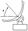
Consider a servomechanism for the azimuth control of an antenna shown in Figure 10.3. The system (cf. Gopal (1993)) has the state vector

and input and output vectors

where  is the angular position of the antenna, is the angular position of the antenna,  is the input voltage applied to the servo motor, and is the input voltage applied to the servo motor, and  is the disturbing torque acting on the motor's shaft. In the following examples we will find the continuous and discrete Kalman estimators. The input is the disturbing torque acting on the motor's shaft. In the following examples we will find the continuous and discrete Kalman estimators. The input  and output and output  noise terms will be assumed to be white, mutually uncorrelated noises with zero-mean values. noise terms will be assumed to be white, mutually uncorrelated noises with zero-mean values.

Figure 10.3. Antenna schematic.
Here is a state-space realization of the antenna mechanism.
In[51]:=
Out[51]=
This defines the noise variances.
In[52]:=
This finds the stationary Kalman gains achieved after an observation of sufficient length. The first input in our antenna system is the only deterministic input, which is specified by the fourth argument to LQEstimatorGains.
In[53]:=
Out[53]=
This is a discrete-time approximation to antenna for some sampling period.
In[54]:=
Out[54]=
Now we let both noise terms have the same intensity.
In[55]:=
This finds the stationary Kalman gain matrix for the discrete-time system.
In[56]:=
Out[56]=
Like most other functions in Control System Professional, LQEstimatorGains accepts both continuous- and discrete-time objects and chooses the appropriate algorithm accordingly.
|