|
10.7 Kalman Estimator
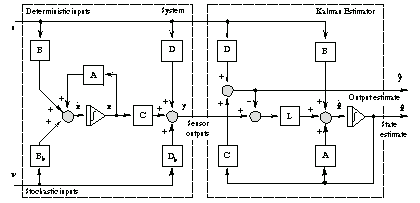
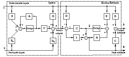
Once the gain matrix  for the Kalman estimator has been found, the estimator can be constructed as a state-space object using KalmanEstimator. The block diagram of the device is shown in Figures 10.4 and 10.5 for continuous and discrete cases, respectively. Notice that the estimator outputs the estimates for both output and state variables of the system, and therefore can be used either as an estimator per se (for example, to form a controller, as described in the following section) or as a filter (see the example later in this section). for the Kalman estimator has been found, the estimator can be constructed as a state-space object using KalmanEstimator. The block diagram of the device is shown in Figures 10.4 and 10.5 for continuous and discrete cases, respectively. Notice that the estimator outputs the estimates for both output and state variables of the system, and therefore can be used either as an estimator per se (for example, to form a controller, as described in the following section) or as a filter (see the example later in this section).

Figure 10.4. Continuous Kalman estimator.

Figure 10.5. Discrete Kalman estimator.


Kalman estimator design.
Consider a two-input, two-output system.
In[59]:=
Out[59]=
Let the estimator gain matrix be symbolic.
In[60]:=ll = {{l}};
This finds the state-space representation for the Kalman estimator assuming that the first output of the system is the sensor output and only the first of the inputs is deterministic. The result agrees with the block diagram in Figure 10.4.
In[61]:=
Out[61]=
Now we create another system that has the same state-space matrices as the pervious one, but is in the discrete-time domain.
In[62]:=
Out[62]=
KalmanEstimator recognizes the discrete-time data object and, consequently, computes the discrete-time estimator. The result satisfies the block diagram in Figure 10.5.
In[63]:=
Out[63]=
Because KalmanEstimator provides estimates for output signals, too, it can be used as a Kalman filter (Figure 10.6). In the rest of this section, we design and try out the Kalman filter, which extracts the useful signal from additive Gaussian noise that masks the angular measurements for the antenna servomechanism (see Section 10.5).

Figure 10.6. Kalman filter connected to a system.
This is again our antenna system.
In[64]:=
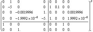
Out[64]=
Recall that the variance of the process noise is q, and the variance of the measurement noise is r. We now make the measurement noise far more intense and will try to filter it out with the Kalman filter.
In[65]:=
This is the estimator gain matrix.
In[66]:=
Out[66]=
Notice that because the process noise was made relatively small and the measurement noise was relatively large compared with the noise in the example in Section 10.5, the relatively smaller gains in the Kalman estimator were achieved. Consequently, the Kalman filter will rely more on re-creating the output signal from the deterministic input using the known system dynamics than on actually processing the noisy sensor output, which is the optimal strategy for noisy measurements.
This is a new object, antenna1, that incorporates another stochastic input through which the measurement noise adds directly to the output. This is done by using the parallel connection with no input connected. The expanded system has three inputs and one output.
In[67]:=
Out[67]=
This finds the Kalman estimator. Note that only the first output of the estimator gives the filtered output of the system (the rest of the outputs give estimates for the state vector; see Figure 10.4).
In[68]:=
Out[68]=
This picks the subsystem we are currently interested in. It contains all the inputs and the first output of the estimator.
In[69]:=
Out[69]=
Then, we connect the expanded system antenna1 and the Kalman filter according to the diagram in Figure 10.7. First we connect the inputs. In the figure, the inputs and outputs are numbered as they appear after this stage.
In[70]:=
Out[70]=

Figure 10.7. Kalman filter connection example.
Finally, we close the feedback loop by connecting the first output of the preceding system with its fourth input (which actually is the first input of the filter). In the composite, the first output corresponds to the output of the system and the second one to the filtered output.
In[71]:=
Out[71]=
To create the normally distributed noise, we will load this standard package.
In[72]:=
Let the length of our simulation sequences be n.
In[73]:=
This creates the process noise vector that has the Gaussian distribution with zero mean and standard deviation as required.
In[74]:=
This is the measurement noise vector.
In[75]:=
This is the sinusoidal input signal.
In[76]:=
We intend to supply no external signal to the summing input  . This prepares a dummy zero signal for this input. . This prepares a dummy zero signal for this input.
In[77]:=
This is where the simulation is performed. The result is a list of output vectors.
In[78]:=
We wish to see how the filter suppresses the measurement noise added to the system output signal y1. The "original" signal (before the addition of noise v) is denoted as y10.
In[79]:=
This plots the signals. We can see that the Kalman filter has quite successfully restored the original signal from the noise.
In[80]:=

|