|
4.1 Symbolic Approach
For the continuous-time system

StateResponse, when supplied with the symbolic input  , attempts to find the solution , attempts to find the solution
 The first term in this equation represents the zero-input response (also called the free, natural, unforced, or homogeneous response) and the second is the zero-state (or particular, forced) response. Once the state response  is found, the output response is found, the output response  can computed directly from the equation can computed directly from the equation

OutputResponse, therefore, calls StateResponse first and then proceeds according to Eq. (4.3). The preceding solution is valid for constant-coefficient matrices  , whereas matrices , whereas matrices  , ,  , and , and  may be time dependent. may be time dependent.
The state response for the discrete-time system
 is computed according to
 and the output response is found by
 Again, matrices  , ,  , and , and  may be time dependent, but matrix may be time dependent, but matrix  may not. may not.


State and output responses to an input function.
For both functions, the input system can be supplied in either state-space or transfer function form; however, the computation is always carried out in the state-space form and the transfer functions are converted to state-space form first. Because matrices  and and  are not needed to compute the state response, their presence in the input system for StateResponse is optional. are not needed to compute the state response, their presence in the input system for StateResponse is optional.
Load the application.
In[1]:=
Consider a transfer function with a simple pole.
In[2]:=
Out[2]=
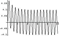
This finds the output response to the sinusoidal input function  . We can see that the first exponential term (the natural response) will vanish, leaving only the harmonic (forced) signal in the output. . We can see that the first exponential term (the natural response) will vanish, leaving only the harmonic (forced) signal in the output.
In[3]:=
Out[3]=
The built-in Mathematica function Plot plots the result on some time interval.
In[4]:=

The zero-input response in Eq. (4.2) or Eq. (4.5) depends on the initial conditions on the state vector  or or  , respectively. By default, StateResponse and OutputResponse assume zero initial conditions. If this is not the case, the initial conditions can be supplied using the option InitialConditions. The typical format is InitialConditions , respectively. By default, StateResponse and OutputResponse assume zero initial conditions. If this is not the case, the initial conditions can be supplied using the option InitialConditions. The typical format is InitialConditions  vector, where vector must have the same length as matrix vector, where vector must have the same length as matrix  . Also acceptable is InitialConditions . Also acceptable is InitialConditions  value, which will cause all state variables to have the same initial value. value, which will cause all state variables to have the same initial value.
Using the option ControlInputs you can effectively cycle through the subsystems that correspond to the specified list of inputs. For ControlInputs  Automatic, StateResponse and OutputResponse apply the input function to all inputs in turn. Another option, ResponseVariable, allows you to name the internal variable if the state or output response should contain unevaluated integral(s) or sum(s). The default value for this option is Automatic, which corresponds to the internal integration variable Tau or summation index K for the continuous- and discrete-time cases, correspondingly. Automatic, StateResponse and OutputResponse apply the input function to all inputs in turn. Another option, ResponseVariable, allows you to name the internal variable if the state or output response should contain unevaluated integral(s) or sum(s). The default value for this option is Automatic, which corresponds to the internal integration variable Tau or summation index K for the continuous- and discrete-time cases, correspondingly.

Specifying initial conditions and the response variable in StateResponse and OutputResponse.
As an example consider the simple production and inventory control model from Brogan (1991):
 which can be represented schematically as shown in Figure 4.1. The model assumes that  and and  are the scheduled production rate and the sales rate, respectively, are the scheduled production rate and the sales rate, respectively,  and and  represent the actual production rate and inventory level, and represent the actual production rate and inventory level, and  is the desired inventory level. is the desired inventory level.

Figure 4.1. Simple production and inventory control system.
Here is the production and inventory control model.
In[5]:=
Out[5]=
Initially the system was in equilibrium, with the production rate  equal to the sales rate and equal to the sales rate and  . We denote . We denote  as x10. At as x10. At  , sales increase by 10 percent. , sales increase by 10 percent.
This finds the state response for the particular value of  . The initial conditions are specified using the option InitialConditions. . The initial conditions are specified using the option InitialConditions.
In[6]:=
Out[6]=
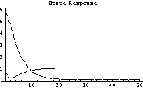
This plots the results for particular values of the initial production rate  and inventory level and inventory level  . To distinguish the graphs for production rate and for inventory level, we set PlotStyle for them differently. The first is plotted as a solid line and the second as a dashed one. . To distinguish the graphs for production rate and for inventory level, we set PlotStyle for them differently. The first is plotted as a solid line and the second as a dashed one.
In[7]:=

We can see that (within this model) keeping initial inventory relatively large allows us to stabilize production rate at a new level.
Note that if multiple input signals are supplied to StateResponse and OutputResponse, the number of signals must be equal to the number of inputs. For multi-input systems, an input signal must be supplied as a vector of functions, but for single-input systems, a function without the List wrapping is also acceptable (in the simulation mode, the same rule of correspondence between the number of input signals and the number of inputs applies—see Section 4.2). If only the response from one or several inputs or outputs must be studied, the function Subsystem (or DeleteSubsystem) may be used to select the subsystem of interest. For further examples when the same input signal is to be applied to all inputs in turn, see Section 4.3.
Here is a two-output system.
In[8]:=
Out[8]=
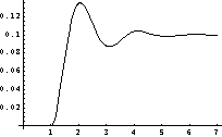
This selects the subsystem associated with the second output and computes the output response to a delayed step function.
In[9]:=
Out[9]=
We can use ComplexExpand to reduce the complex exponentials to the trigonometric functions.
In[10]:=
Out[10]=
This simplifies the result.
In[11]:=
Out[11]=
This is a plot of the response.
In[12]:=

Here is a discrete-time system.
In[13]:=
Out[13]=
In this input vector, the components are a ramp function and a decaying exponential  both sampled at a unit-time interval. both sampled at a unit-time interval.
In[14]:=
Out[14]=
This is the state response for the particular set of initial conditions. Since k is a real valued parameter, the expression can be simplified with ComplexExpand.
In[15]:=
Out[15]=
Once the state response vector is available, the output response can be found.
In[16]:=
Out[16]=
The same result can be obtained directly.
In[17]:=
Out[17]=
|