Fitting Data to Nonlinear Models

Enable JavaScript to interact with content and submit forms on Wolfram websites. Learn how

Chapter 5

Fitting Data to Nonlinear Models

One of the most difficult topics in all of data analysis in the physical sciences is fitting data to nonlinear models. Often such fits require large computational resources and great skill, patience, and intuition on the part of the analyst. These difficulties are one of the reasons that, as we shall see, the whole topic of spectral line shapes is still a very active subject of research spanning the fields of chemistry, physics, astronomy, and more. In addition, computational methods of nonlinear fitting are still a current research topic in computer science.

However, since sometimes nature really is nonlinear, such fits are often unavoidable, and the principles and some tools for nonlinear fitting are the topics of this chapter. The main EDA program introduced here is FindFit, which accomplishes fits to arbitrary models.

FindFit is similar to the NonlinearFit function in the Statistics`NonlinearFit` package which is standard with Mathematica. The primary differences are that FindFit: (1) recognizes EDA's data format, including errors in both coordinates; (2) estimates errors in fit parameters; (3) by default displays graphical information about the fit; and (4) uses an algorithm that has been optimized for speed and stability for the types of nonlinear fits commonly performed in the physical sciences and engineering.

5.1 Introduction

5.1.1 Overview of FindFit

The previous chapter, "Fitting Data to Linear Models by Least-Squares Techniques," introduced the distinction between linear and nonlinear models. To briefly review, the terms refer to the way in which the parameters to which we are fitting enter into the model.

In this chapter we discuss nonlinear models and the EDA program FindFit that can often find a reasonable fit to them.

Recall that if sos is the sum of the squares of the residuals, then we are seeking the minimum in its value. If we are fitting to parameters a[0], a[1], ... , a[m], the answer is found by solving a set of simultaneous equations.

This, in general, can be done analytically, provided the model to which we are fitting is linear in the parameters. Similarly, when there are explicit errors in the data, we form the chi-squared, , and we solve the corresponding equations.

This again will be analytic for a linear fit.

For a nonlinear fit, no such analytic solutions are possible, so iteration is required to find the minimum in the sum of the squares or the chi-squared.

If we imagine a plot of the value of the sum of the squares or the chi-squared as a function of the parameters to which we are fitting, in general for a nonlinear fit there may be many local minima instead of one big one, as is the case for linear fitting. For example, if we are fitting to two parameters, param1 and param2, the chi-squared as a function of the values of the parameters might have two or more local minima.

In[1]:=

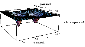
Thus, a nonlinear fitter must usually start off with initial values close to the real minimum.

The general technique for iteration, "steepest descent," is analogous to the following situation. "It was a dark and stormy night." Foggy too. You are on the side of a hill and want to find the valley. So, you step in the direction in which the slope goes down, and continue moving in the direction of the local definition of "down" until you are in the valley. Of course, if you take giant steps you might step over the next hill and end up in the wrong valley. And when you get close to the bottom of the valley you will want to start taking baby steps. The Levenberg-Marquardt algorithm used by many nonlinear fitters, including FindFit by default, is essentially some clever heuristics to define giant steps and baby steps.

If the data has noise, which is almost a certainty for real experimental data, then there is a further difficulty. We can take two sets of data from the same apparatus using the same sample, fit each dataset to a nonlinear model using identical initial values for the fit parameters, and get very different final fits. This situation leads to ambiguity about which fit results are "correct."

5.1.2 Providing Initial Parameter Values to FindFit

As already mentioned, unless we are fitting to a very simple model, FindFit must be provided with initial estimates of the parameters.

We will first fit to a simple model where no such parameter estimates are necessary.

In[2]:=

In[3]:=

In[4]:=

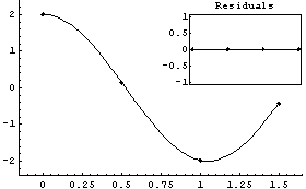
Out[4]=

Actually, when not given initial values FindFit starts with initial values for the parameters, here a and b, equal to 1.

Now the syntax of the call to FindFit is given.

Here ind is the name of the independent variable in model. Also note that this model is nonlinear in the parameters to which we are fitting, param1 ... paramM.

The EDA`FindFit` package includes a Gaussian function.

In[5]:=

We will use it to generate some data.

In[6]:=

We examine the data with EDAListPlot.

In[8]:=

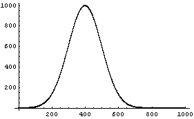
We fit the data using FindFit; the fit takes a few seconds to complete.

In[9]:=

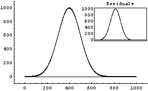
Out[9]=

This result is ridiculous. What has happened is that FindFit thinks it has found a local minimum in the sum of the squares at these silly values.

Repeating the fit with reasonable initial guesses of the parameters gives a much better result.

In[10]:=

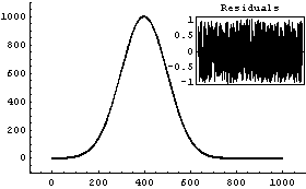
Out[10]=

Finding good initial values is sometimes subtle. As an example, we generate some made-up data for three peaks with a Lorentzian shape using the Lorentzian function supplied with the EDA`FindFit` package.

In[11]:=

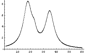
It is difficult to see the small peak on the shoulder of the leftmost peak, or to provide initial estimates for its values. However, we can see the peak and probably make some sensible guesses of its parameters.

Despite the claims sometimes seen in glossy advertisements, there is no known software that can find and estimate peaks for data such as this as well as a human expert. This is in part because of the great ability of the human visual system to be an intuitive integrator.

Almost all versions of the notebook front end for Mathematica include a provision to use our visual ability. We can display a graph of the data and use the mouse to point to a desired location on the graph; for Windows versions we must hold down the key. The coordinates will be displayed in the notebook window, and can also be copied out using the cut-and-paste facility; consult the manual for your version of the notebook to discover how to do this. For example, here we load and examine a part of a nuclear spectrum.

In[14]:=

In[15]:=

In[16]:=

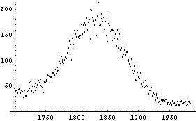
Using the mouse we can pick out the coordinates of the maximum, the points on the peak corresponding to roughly one-half the maximum, and so on. So, the position of the peak is found.

In some earlier versions of the Windows front end, if the notebook is closed and then reopened, the coordinates will be returned in PostScript units instead of the actual units of the plot; rerendering the plot works around this bug.

Finally, for simple spectra EDA supplies a function FindPeaks, which can sometimes provide initial guesses of the number of peaks and their parameter values close enough for FindFit. The function is described in Section 8.3.

5.1.3 Comparing LinearFit and FindFit

Although FindFit is intended for fitting to nonlinear models, it can also find the minimum in the sum of the squares or the chi-squared for linear models, although more slowly than LinearFit.

For example, here we repeat a fit from Chapter 4.

In[17]:=

Out[17]=

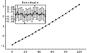
Using FindFit yields the same result.

In[18]:=

Out[18]=

Although not an issue for this small data set, FindFit took about four times as long as LinearFit.

Recall from the chapter on linear fitting that if the data have explicit errors in both coordinates, the effective variance technique makes the fit essentially nonlinear unless the model is a straight line. Thus, in this case LinearFit iterates until it finds a minimum in the chi-squared. When there are errors in both coordinates, FindFit also calculates the error in the dependent variable based on the effective variance. However, although there is a fairly comprehensive literature on using this technique in linear fits, the main justification for using effective variances in nonlinear fits is based only on a series of experiments in which it was found that the algorithm of FindFit would produce reasonable results most of the time.

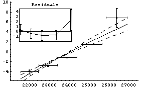
We repeat another fit from the chapter on linear models.

In[19]:=

Out[19]=

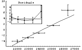
FindFit gives a similar result if started sufficiently close to the "final" values.

In[20]:=

Out[20]=

For the above results, FindFit appears to have done a poorer job of estimating the errors in the fit parameters than LinearFit.

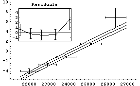
Another difference between the two fits above is that, by default, the graphs produced by LinearFit display the errors in the fit parameters, while the graphs produced by FindFit do not. This is because for many nonlinear fits, sorting out how to combine the various error terms is problematic. To display the fit errors, the UseFitErrors option (discussed in Section 5.3.2.2) may be set to True.

In[21]:=

Out[21]=

Note that as opposed to the plot produced by LinearFit, here the lines representing the errors in the fit parameters are parallel. This is an artifact of a heuristic used by the FindFit package to combine the two terms; the heuristic is often reasonable for true nonlinear fits.

As a final comparison between LinearFit and FindFit, we load and examine some data on oscillations in interneuron networks.

In[22]:=

In[23]:=

In[24]:=

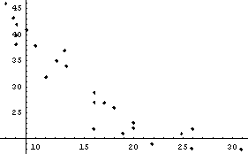
The data appears to be modeled by an exponential relationship.

This is nonlinear in the parameters a and b. However, as mentioned in the previous chapter, we can linearize the relationship by taking the logarithm of both sides.

Thus, we form a data set of {ipscTau, Log[frequency]}.

In[25]:=

We fit this transformed data to a straight line.

In[26]:=

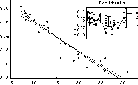
Out[26]=

Thus b = - 0.0424 ± 0.0033 in (. Although there are problems with the above fit, which are discussed below, we will calculate a and its errors using the Datum construct discussed in Chapter 3.

In[27]:=

Out[27]=

Using FindFit, we can fit directly to the exponential.

In[28]:=

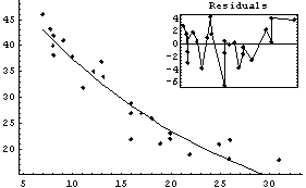
Out[28]=

The two fits are similar, and both show some problems in the residuals. Also, FindFit seems more confident about the uncertainties in the values of the fit parameters, probably without justification. The difference in the SumOfSquares is because of the different values being used for the dependent variable of the data.

One likely reason for the problems here is that the data does not seem to asymptotically approach zero, as assumed by our model, but some other value c.

Fitting to this model seems to confirm our hypothesis.

In[29]:=

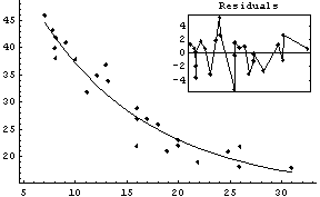
Out[29]=

This essentially duplicates a fit presented by the experimenters in their original paper.

The model can be linearized as follows.

Thus, we can form another data set in which we subtract 13.8 from each value of frequency before taking the logarithms.

In[30]:=

We fit this to a straight line.

In[31]:=

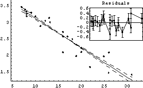
Out[31]=

Thus, a can be calculated.

In[32]:=

Out[32]=

This number is within errors of the result found by FindFit.

Of course, without FindFit or some other nonlinear fitter available, it would be difficult to get an objective estimate of the value that should be subtracted from each value of the dependent variable frequency.

Also, although not an issue here, this sort of linearization procedure can introduce biases in the values of the estimates of the fit parameters; this is discussed further in Chapter 8.

5.1.4 References

Philip R. Bevington, Data Reduction and Error Analysis (McGraw-Hill, 1969), Chapter 11. A classic introduction to nonlinear fitting techniques

Xiang Ouyang and Philip L. Varghese, Applied Optics 28 (1989), p. 1538. A discussion of a popular Fourier transform-based algorithm for fitting spectra to Galatry and Voigt profiles

William H. Press, Brian P. Flannery, Saul A. Teukolsky, and William T. Vetterling, Numerical Recipes: The Art of Scientific Computing or Numerical Recipes in C: The Art of Scientific Computing (Cambridge Univ. Press), Section 14.4. A good brief introduction to nonlinear fitting and the Levenberg-Marquardt algorithm used by FindFit

A.P. De Weljer, C.B. Lucasius, L. Buydens, G. Kateman, H.M. Heuvel, and H. Mannee, Anal. Chem. 66 (1994), p. 23. An illuminating discussion of the research into fitting to curves using neural networks, this article also has a good review of some of the problems with conventional techniques

5.2 Examples

5.2.1 Fitting to a Single Peak with a Background

We begin by loading and examining some data that was briefly examined in Section 5.1.2.

In[1]:=

In[2]:=

In[3]:=

In[4]:=

The theoretical prediction for the peak is that it should be a Gaussian, so part of the model for the fit will be the Gaussian function included in the EDA`FindFit` package.

In[5]:=

We also note that there is a background under the peak, that is, counts in addition to the Gaussian peak. We will approximate the background as a straight line with the following slope.

In[6]:=

Out[6]=

Here the numbers in the calculation are based on values obtained by pointing and clicking at the left- and right-hand sides of the plot of the data with the mouse. We calculate the intercept.

In[7]:=

Out[7]=

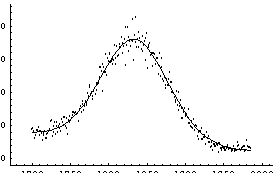
From the plot of the data we estimate the center of the peak to be at channel 1830, and the amplitude above the background is about 140 counts. The full width at half-maximum is about 90 channels, so we will try an initial value for sigma of 45 channels.

Since we are going to use a[0] and a[1] as names for fit parameters, we must clear the definitions we have just made for them.

In[8]:=

Now we fit to the data.

In[9]:=

Out[9]=

Note that the Reweight option, which is True by default for LinearFit, is False by default for FindFit. Section 5.3.1.9 discusses this further.

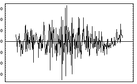
Note also that because all four quadrants of the plot of the data and the fit contain significant amounts of data, FindFit displays the plot of the residuals separately.

Here is the syntax of the call to FindFit.

The model is the model to which we are fitting and ind is the independent variable. The params can be a list of the parameter names.

More often params is a list of {parameter name, initial value} pairs.

The world will end if model contains undefined arguments in addition to ind and those named in params.

Other forms of parameter specification include {name, min, start, max}, which causes FindFit to begin parameter name at start and not allow it to go below min or above max. Or the parameter can be specified as {name, min, max}, in which case the value starts at (min + max)/2.

Note that in comparison to fits you may have done using LinearFit, FindFit is very slow.

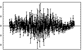
From the theory of nuclear physics, we expect the error in the number of counts in each channel to be Sqrt[counts]. Thus, we form a new data set with these errors included.

In[10]:=

We fit to this new data set.

In[11]:=

Out[11]=

Although the error bars in the data have obscured the curve representing the fit, the residuals and the ChiSquared per DegreesOfFreedom show that the fit is reasonable, except perhaps on the far right-hand side.

There is another sort of bell-shaped curve that high-energy physicists usually call a "Breit-Wigner". The same curve is usually called a "Lorentzian" by spectroscopists. The EDA`FindFit` package includes a BreitWigner function.

In[12]:=

We can compare the shape of a Breit-Wigner to a Gaussian.

In[13]:=

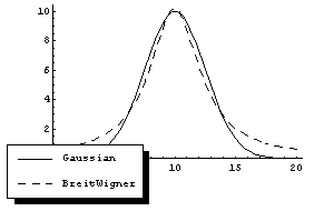
Note that, consistent with a common convention, BreitWigner does not take the maximum amplitude as an argument, but instead the total area under the curve. If the peak in the Cobalt-60 data is a Breit-Wigner, this corresponds to the total number of counts in the peak. The total number of counts in the data, peak plus background, can be calculated.

In[15]:=

Out[15]=

Also, the width is specified by the full width at the half-maximum, not the standard deviation. We fit the Cobalt-60 data with errors to a Breit-Wigner plus a linear background.

In[16]:=

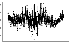
Out[16]=

Because of the possibility that FindFit fell into the wrong minimum in the chi-squared, caution must be used in rejecting the model (i.e., a Breit-Wigner plus background) because of a large ChiSquared per DegreesOfFreedom. Nonetheless, the residuals seem to be saying clearly that the data does not match a Breit-Wigner.

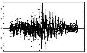
For the fit to a Gaussian, there are some signs of a problem at higher values of the channel. We try to account for that by adding a quadratic term to the background.

In[17]:=

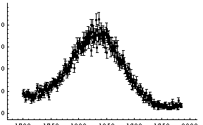
Out[17]=

This seems to be much better. Note that the values of the parameters for the background have changed dramatically by the addition of the second-order term.

Finally, we can compare the total number of counts in the data, 24057, to the total predicted from the fit.

In[18]:=

Out[18]=

Whether or not this number is close to the experimental number cannot be answered until we do some error analysis. We can find the contributions to this number from the background and the Gaussian, including errors, using some tools discussed in Chapter 3.

We ignore the quadratic term in the background. Using the Datum construct, we can find the counts and error in the counts due to the background.

In[19]:=

Out[19]=

We use the fact that the Gaussian is essentially zero at both the left and right of the data, so we can use the full normalization of the Gaussian to calculate the counts under the peak.

In[20]:=

Out[20]=

Thus, the total number of counts predicted by the fit is calculated.

In[21]:=

Out[21]=

This compares well with the experimental value of 24057.

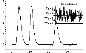
5.2.2 Fitting to Three Peaks with No Background

A common line shape in the study of infrared absorption and emission is called a Galatry profile. The EDA`FindFit` package includes a function for this shape.

In[22]:=

We will use this function to generate some made-up data of three Galatry peaks.

In[23]:=

In[25]:=

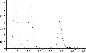
We fit to this data.

In[26]:=

Out[26]=

However, you should be aware that this fit pushed FindFit pretty hard. Not only is the fit very sensitive to the initial values, but on a very fast Linux machine running a 500 Mhz Xeon processor the fit took over 15 seconds of cpu to perform. Further, many of the fitted parameters are zero within calculated errors. This is why specialized software to solve these sorts of problems has been written. See Ouyang and Varghese, listed in the references, Section 5.1.4, for an example of a technique for fitting this particular type of spectrum.

5.3 Options, Utilities, and Details

There are many options to FindFit that control both how it does the fit and what it returns. These are discussed in Section 5.3.1.

The package also includes programs that are used by FindFit, but may also be used directly. These are the topic of Section 5.3.2, which also discusses some convenience functions of various peak shapes.

First we load EDA.

In[1]:=

5.3.1 Options to FindFit

The options and default values used directly by FindFit are given by using Options.

In[2]:=

Out[2]//TableForm=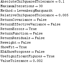

Below, we first discuss the Method option, followed by the other options to FindFit in order.

In addition, if ShowFit is set to True, the default, FindFit, uses the function ShowFitResult. This function is discussed in Section 5.3.2. Options to ShowFitResult given to FindFit are passed to that function.

If FindFit is called with ReturnFunction set to True, or if the ShowFit option is set to True (the default) the function ToFitFunction is called. This function is discussed in Section 5.4.2. Options to ToFitFunction given to FindFit are passed to that function.

5.3.1.0 The Method Option

In many cases, FindFit by default uses the Mathematica built-in function FindMinimum with a LevenbergMarquardt method. FindFit can use other methods, controlled with a Method option. Valid values include Gradient, Newton, and QuasiNewton, all of which are passed to FindMinimum.

FindFit has its own Levenberg-Marquardt algorithm, coded in a form very similar to that described by Press et al. in Numerical Recipes, §14.4. When Method is set to EDALM this code will be used to find the fit. EDALM will always be used when either there are explicit errors in both coordinates of the data or when the Reweight option discussed below has been set to True, or if the model being fit to is linear; in all of these cases this behavior is invisible unless the ShowProgress option discussed below is set to True.

Here is an illustration. First we fit Cobalt60Data to a Gaussian plus linear background without reweighting; we also suppress the graphs of the fit by using the ShowFit option.

In[3]:=

Out[3]=

Now we reweight the data.

In[4]:=

Out[4]=

Finally, we repeat the above fit but observe its progress. The fourth line of the progress report tells us that the method has been changed.

In[5]:=

Out[5]=

The EDALM method is the only one which uses the following options: AbsoluteChiSquaredTolerance, MaximumIterations, RelativeChiSquaredTolerance, and ValueTolerance.

5.3.1.1 The AbsoluteChiSquaredTolerance Option

When FindFit is performing a fit using the EDALM algorithm discussed in Section 5.3.1.0, it uses three separate tests to determine if a fit has converged to a final value. The AbsoluteChiSquaredTolerance option is used by one of those tests.

If the chi-squared (or the sum of the squares if there are no explicit errors in the data) is decreasing and, in the current iteration, its value is less than the value in the previous iteration by AbsoluteChiSquaredTolerance, the fit is judged to have converged.

If there are declared errors in the data being fit, so that the test is comparing chi-squared statistics, the default value of 0.1 for this option is usually reasonable. If there are no declared errors, so the test is comparing the sum of the squares of the residuals, then the actual value of the sum of the squares depends on the magnitude of the values of the dependent variable. In this case some adjustment of the value of AbsoluteChiSquaredTolerance may be appropriate.

For information on the other two tests used by FindFit to determine convergence, see the discussion of the RelativeChiSquaredTolerance and ValueTolerance options in 5.3.1.3 and in 5.3.1.13, respectively.

5.3.1.2 The MaximumIterations Option

As discussed above, FindFit uses an iterative technique to try to determine the minimum in the chi-squared or sum of the squares. The MaximumIterations option controls the number of iterations FindFit will attempt before giving up.

When FindFit gives up, it issues a warning message, but also presents the result of the fit just as if it had converged. For example, here we repeat a fit we performed in Section 5.1.3, but we restrict the number of iterations to less than that required by FindFit to achieve convergence.

In[6]:=

Out[6]=

5.3.1.3 The RelativeChiSquaredTolerance Option

When FindFit is performing a fit using the EDALM algorithm discussed in Section 5.3.1.0, it uses three separate tests to determine if a fit has converged to a final value. The RelativeChiSquaredTolerance option is used by one of those tests.

If the chi-squared (or the sum of the squares if there are no explicit errors in the data) is decreasing, and the value of the previous iteration minus the current value divided by the previous value is less than the value of RelativeChiSquaredTolerance, then the fit is judged to have converged.

If there are declared errors, so that the test is comparing chi-squared statistics, the default value of 0.005 for this option is usually reasonable. If there are no declared errors, so the test is comparing the sum of the squares of the residuals, then the actual value of the sum of the squares depends on the magnitude of the values of the dependent variable; in this case some adjustment of the value of RelativeChiSquaredTolerance may be appropriate.

For information on the other two tests used by FindFit to determinate convergence, see the discussion of the AbsoluteChiSquaredTolerance option and of the ValueTolerance option in 5.3.1.1 and in 5.3.1.13, respectively.

5.3.1.4 The ReturnCovariance Option

If the ReturnCovariance option is set to True, then FindFit returns the full covariance matrix of the fit in addition to other rules about the result.

A discussion of the meaning of the covariance matrix is in Section 4.4.18.

5.3.1.5 The ReturnEffectiveVariance Option

When both coordinates have errors, FindFit uses an "effective variance" technique. This method is discussed in Section 4.1.3.

If the ReturnEffectiveVariance option to FindFit is set to True, then the program returns the values of the effective variance in addition to other rules about the result.

This option is identical to the option of the same name used by LinearFit.

5.3.1.6 The ReturnErrors Option

By default, FindFit calculates and returns the errors in the fit parameters. It also uses these errors to adjust the significant figures in the values of the parameters. If ReturnErrors is set to False, no errors are returned and no significant figure adjustment is performed.

For example, here we repeat a fit performed before in this chapter, one with and the other without ReturnErrors set to True. We also set ShowFit to False to suppress the graphs of the fit.

In[7]:=

Out[7]=

In[8]:=

Out[8]=

This option is identical to the option of the same name used by LinearFit.

5.3.1.7 The ReturnFunction Option

Be default, FindFit returns a set of rules for the result of the fit. By setting ReturnFunction to True, FindFit instead returns a function of the independent variable.

For example, here we repeat a fit performed a few times already in this section, but with ReturnFunction set to True. We also set ShowFit to False to suppress the graphs of the fit.

In[9]:=

Out[9]=

This option is identical to the option of the same name used by LinearFit.

5.3.1.8 The ReturnResiduals Option

If set to True, the ReturnResiduals option causes FindFit to return the residuals of the fit along with the other results of the fit.

This option is identical to the option of the same name used by LinearFit.

5.3.1.9 The Reweight Option

When the data has no explicit errors, FindFit finds the minimum in the sum of the squares of the residuals. However, if the scatter in the data points can be considered to be random and statistical then it is often reasonable to assume that the effective error in the dependent variable is given by PseudoErrorY.

The Reweight option is identical to the option of the same name used by LinearFit except that by default it is True for LinearFit, but False for FindFit. This is because in a nonlinear fit, reweighting the data can change the values of the parameters to which we are fitting. This is not true for a linear fit, where reweighting only affects the calculated errors in those parameters.

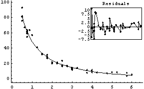
Here is an example. ChwirutData is ultrasonic calibration data.

In[10]:=

The data can be fit to:

and the "certified" values of the parameters are:

Here are the results of fitting the data.

In[11]:=

Out[11]=

Although the values of the parameters from the fit are close to the certified values, the errors are quite different from the certified values. Turning on reweighting makes the errors close to the certified values.

In[12]:=

Out[12]=

You may wish to know that Mathematica supplies nonlinear fitters, such as NonlinearRegress in the standard Statistics`NonlinearFit` package, which use reweighting by default and are optimized for those types of fits. EDA's FindFit is optimized for the case when explicit errors are given in one or both coordinates of the data.

5.3.1.10 The ShowFit Option

Setting ShowFit to False suppresses the display of the graphical information about the fit. As discussed in Section 5.3.2.1, the graphs can be created later from the result returned by FindFit.

This option is identical to the option of the same name used by LinearFit.

5.3.1.11 The EDAShowProgress Option

Setting EDAShowProgress to True causes FindFit to print information about its progress in performing the fit. This option is identical to the one of the same name used by LinearFit, although for FindFit the information is much more verbose and more often of use in finding the "best" fit of the data to a model.

Here we repeat a fit done a few times already in this section, setting ShowProgress to True and setting ShowFit to False to suppress the graphs of the fit.

In[13]:=

Out[13]=

Note that the final iteration satisfied two of the three possible criteria for convergence. This is common when FindFit has found a true minimum in the sum of the squares.

5.3.1.12 The UseSignificantFigures Option

As discussed in Chapter 3, in the physical sciences specifying the error associated with a quantity essentially defines what the significant figures of that quantity are. By default, FindFit uses this definition of significant figures in returning the value of fit parameters. The UseSignificantFigures option allows this default behavior to be turned off. For example, here we repeat a fit we have already done a few times.

In[14]:=

Out[14]=

In[15]:=

Out[15]=

Now the estimated errors in the fitted parameters have not been used to adjust the number of significant figures displayed for either the values or the errors in those parameters.

In Section 5.3.1.9 above, we were comparing a fit to ChwirutData to "certified values." The fit result was as follows.

In[16]:=

Out[16]=

The certified values are:

Turning off significant figure adjustment allows us to compare the result of FindFit to the certified values more carefully.

In[17]:=

Out[17]=

This UseSignificantFigures option is identical to the option of the same name used by LinearFit.

5.3.1.13 The ValueTolerance Option

When FindFit is performing a fit using the EDALM algorithm discussed in Section 5.3.1.0, it uses three separate tests to determine if a fit has converged to a final value. The ValueTolerance option is used by one of those tests.

If the chi-squared or sum of the squares is decreasing, and the maximum of the absolute value of the change in the fit parameters is less than ValueTolerance, the fit is judged to have converged. The default value is 0.002.

For information on the other two tests used by FindFit to determinate convergence, see the discussion of the AbsoluteChiSquaredTolerance and RelativeChiSquaredTolerance option in Section 5.3.1.1 and Section 5.3.1.3, respectively.

5.3.2 Other Routines in the FindFit Package

5.3.2.1 The ShowFitResult Routine

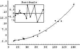
By default FindFit uses the program ShowFitResult to display the results of a fit. If we have the results of FindFit, we can use ShowFitResult to display it. We will demonstrate with GanglionData as used above.

In[18]:=

Out[18]=

Now we display the results of the fit.

In[19]:=

Out[19]=

Note that ShowFitResult returns a Graphics object. This can be convenient if you wish to print the graphic, since the Graphics object is not returned by FindFit itself.

Note that the syntax and functionality of ShowFitResult are very similar to that of ShowLinearFit in the EDA`LinearFit` package.

By default, ShowFitResult tries to find a quadrant in the data-fit graph in which to place the residual plot. If no such quadrant can be found, the residual plot is displayed separately. Setting ResidualPlacement to Separate causes the residual plot to always be displayed separately. ResidualPlacement can also be set to an integer between 1 and 4, which causes the residual plot to be placed in that quadrant of the data-fit plot.

In[20]:=

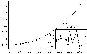
Out[20]=

If ResidualPlacement is set to None, no residual plot is displayed.

By default, the plot of the fit results only spans the values of the data. An Extrapolate option causes the values of the independent variable to be in the range specified by the option.

In[21]:=

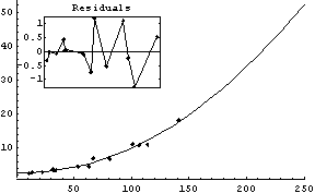
Out[21]=

Internally, ShowFitResult uses EDAListPlot, Plot, and ToFitFunction. Options given to ShowFitResult for these are passed to the appropriate program. In addition, ShowFitResult itself uses only the two options ResidualPlacement and UseSignificantFigures.

There can be some minor differences between the graphs displayed by FindFit and those displayed by ShowFitResult. For example, if the data set has no explicit errors and the Reweight option is set to True in the call to FindFit, then the PseudoErrorY is used in the calculation of the errors in the residuals by FindFit. ShowFitResult is unaware of this, and will then have slightly different errors in the residual graph. By specifying ReturnResiduals to True in the call to FindFit, the "better" numbers will be used by ShowFitResult.

We give an example by fitting GanglionData with the Reweight option.

In[22]:=

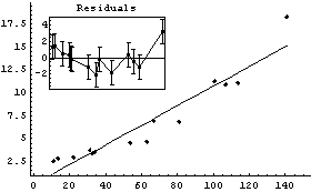
Out[22]=

Next we use ShowFitResult on result.

In[23]:=

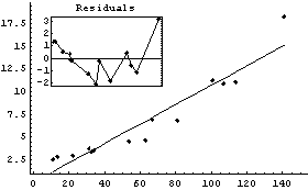
ShowLinearFit does not show the errors in the residuals due to the PseudoErrorY term.

We can have FindFit explicitly return the residuals.

In[24]:=

Out[24]=

We see that the PseudoErrorY has led to an error in each of the residuals. ShowFitResult will display these in this case.

In[25]:=

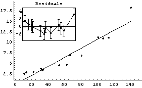
Similarly, if the data set has errors in both coordinates, FindFit uses the effective variance in calculating the errors in the residuals. In this case also, specifying ReturnResiduals as True in the call to FindFit will cause ShowFitResult to be slightly more correct.

5.3.2.2 The ToFitFunction Routine

ShowFitResult, discussed previously, uses the function ToFitFunction to graph the results of the fit. FindFit also directly calls ToFitFunction if the option ReturnFunction is set to True.

The function may also be called directly. We repeat a fit we have done before.

In[26]:=

Out[26]=

We pass the result to ToFitFunction.

In[27]:=

Out[27]=

ToFitFunction is similar to the ToLinearFunction function supplied in the EDA`LinearFit` package, but somewhat more general. One difference is that when the fit parameters have errors, by default ToFitFunction does not return two functions. In contrast, ToLinearFunction will return two functions, the first being the result of the fit and the second the estimated errors in the function. ToFitFunction can return this second "error function" if the UseFitErrors option is set to True.

In[28]:=

Out[28]=

5.3.3 Peak Shape Routines

The EDA`FindFit` package includes some convenience functions to define peak shapes. They are BreitWigner, Galatry, Gaussian, Lorentzian, PearsonVII, RelativisticBreitWigner, and Voigt.

5.4 Summary of the FindFit Package

In[1]:=