|
Examples
Generation of Random Numbers
One standard normal variable
Now we will develop a short Mathematica program to generate random numbers from the standard normal distribution using a well-known method.
First we generate two random variables from the uniform distribution on the interval [-1 , 1].
In[1]:=r = Table[Random[Real, {-1, 1}], {2}]
Out[1]=
We repeat this until the sum of the squares of these two numbers is less then 1.
In[2]:=(s = 1;
While[s >= 1,
r = Table[Random[Real, {-1, 1}], {2}];
s = r . r
];)
We get a pair of independent standard normal variables.
In[3]:=r Sqrt[-2 Log[s] / s]
Out[3]=
We pick the first one.
In[4]:=First[r] Sqrt[-2 Log[s]/s]
Out[4]=
Now we collect these steps into a program chance[ ].
In[5]:=chance[ ] :=
Module[{r, s = 1},
While[s >= 1,
r = Table[Random[Real, {-1, 1}], {2}];
s = r . r
];
First[r] Sqrt[-2 Log[s] / s]
]
We generate a list of 2000 random numbers from the standard normal distribution.
In[6]:=data = Table[chance[ ], {2000}];
Now we will check how good our random number generator is. We will use the function BinCounts from the standard statistics package.
In[7]:=Needs["Statistics`DataManipulation`"]
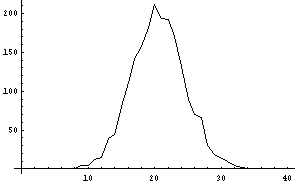
We first tabulate the frequencies in order to compare them with the predicted frequencies.
In[8]:=freq = BinCounts[data, {-5, 5, .25}];
This explains what BinCounts does.
In[9]:=?BinCounts
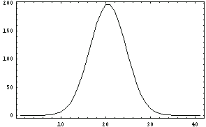
This is the graph of the frequencies.
In[10]:=g1 = ListPlot[freq, PlotJoined -> True];
We load the Options subpackage to get the function Norm.
In[11]:=
In[12]:=

We compute the predicted frequencies.
In[13]:=predfreq = Table[2000 (Norm[x+.25] - Norm[x]),
{x, -5, 5, .25}];
This is the corresponding plot.
In[14]:=g2 = ListPlot[predfreq, PlotJoined -> True];
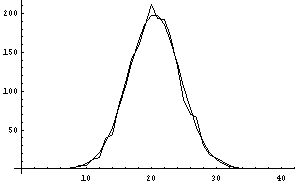
One way to compare the graphs is to display them together.
In[15]:=Show[g1, g2];
Two correlated standard normal variables
We can modify our program to generate a pair of standard normal variables for a given correlation coefficient rho.
In[16]:=chance[rho_] :=
Module[{r1, r2, s = 1},
While[s >= 1,
{r1, r2} = Table[Random[Real, {-1, 1}], {2}];
s = {r1, r2} . {r1, r2};
];
Sqrt[-2 Log[s] / s] *
{r1, rho r1 + Sqrt[1 - rho^2] r2}
]
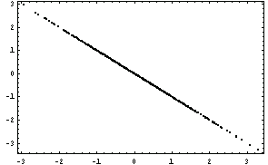
We generate 500 pairs of random numbers with -1.0 as the correlation coefficient.
In[17]:=m = Table[chance[-1.0], {500}];
Here is the corresponding graph.
In[18]:=ListPlot[m];
We generate 500 pairs of random numbers with -0.8 as the correlation coefficient.
In[19]:=m = Table[chance[-0.8], {500}];
Here is the corresponding graph.
In[20]:=ListPlot[m];
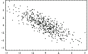
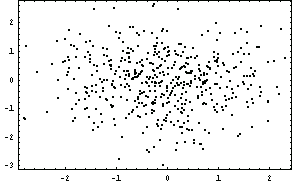
We generate 500 pairs of random numbers with 0. as the correlation coefficient.
In[21]:=m = Table[chance[0.], {500}];
Here is the corresponding graph.
In[22]:=ListPlot[m];
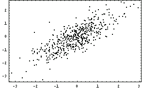
We generate 500 pairs of random numbers with 0.8 as the correlation coefficient.
In[23]:=m = Table[chance[0.8], {500}];
Here is the corresponding graph.
In[24]:=ListPlot[m];
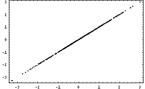
We generate 500 pairs of random numbers with 1.0 as the correlation coefficient.
In[25]:=m = Table[chance[1.0], {500}];
Here is the corresponding graph.
In[26]:=ListPlot[m];
Markowitz Efficient Portfolio
First we load the subpackage.
In[27]:=<< Finance`Examples`
This package modifies the mean and covariance functions so that they can be used in the multivariate case. The other functions will be explained below.
In[28]:=?Finance`Examples`*
CovarianceMatrix MeanVector PortfolioVariance
EfficientFrontier PortfolioMean ShowWeights


Auxiliary functions.
The file stocks1.ret contains the returns of five stocks in 24 consecutive months. The first line just contains the number of stocks, the second line contains the time unit and the stocks' tickers, and the remaining lines start with the month number followed by the returns of stocks.
5
Month AMR BS UTX WX Z
1 11.594 1.515 -1.579 -9.360 -0.408
2 22.078 5.299 9.947 7.578 0.000
3 -8.511 -8.000 9.446 -16.327 0.694
4 -3.488 0.395 5.164 -8.571 -3.862
5 -9.639 -9.764 -3.571 -18.243 -10.949
6 -12.000 6.195 -0.943 -11.570 -8.197
7 -10.606 -0.417 -7.619 -8.441 -6.786
8 -1.695 -6.276 11.856 -8.220 -13.725
9 -12.069 -9.091 -3.286 -10.227 -2.273
10 27.451 15.000 11.186 -3.797 2.791
11 -21.538 -4.465 6.550 -4.021 -8.140
12 -19.608 -6.132 8.750 12.676 -5.063
13 48.780 27.156 4.215 12.500 35.200
14 19.672 -2.372 7.355 15.271 12.121
15 1.370 15.190 13.889 18.000 -0.901
16 4.054 15.751 17.073 -0.847 18.548
17 -15.584 -9.810 1.042 23.884 -10.958
18 3.077 4.270 20.833 4.196 14.912
19 -4.478 -6.485 -7.543 -4.027 -5.058
20 4.688 11.679 3.263 -6.333 4.918
21 -11.940 -7.285 3.189 -18.939 -3.125
22 -1.695 -3.214 -7.506 -2.856 27.742
23 15.517 0.369 -3.580 5.882 16.026
24 5.970 -1.866 -7.250 -0.926 -2.762
25 11.268 26.616 15.903 16.822 13.295
We have to open a stream to read in the data.
In[29]:=stream = OpenRead[ToFileName[{"Finance","Data"}, "stocks1.ret"]];
We get the number of assets.
In[30]:=n = Read[stream, Number]
Out[30]=
We read in the tickers.
In[31]:=tickers = Rest[Read[stream, Table[Word,{n+1}],
RecordSeparators -> {"\n"," ", "\t"}]]
Out[31]=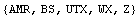
We read in the rest of the data.
In[32]:=aux = Transpose[Partition[ReadList[stream, Number], n+1]];
Finally we close the stream.
In[33]:=Close[stream];
This defines lists of the months and the stocks' returns.
In[34]:={months, returns} = {First[aux], Transpose[Rest[aux]]};
These are the means of the returns for each stock.
In[35]:=mean1 = MeanVector[returns]
Out[35]=
We can display this in tabular form.
In[36]:=PaddedForm[TableForm[mean1,
TableHeadings -> {tickers},
TableAlignments -> {Right}], {6, 3}]
Out[36]//PaddedForm=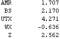
Next we compute the covariance matrix.
In[37]:=cov1 = CovarianceMatrix[returns];
In[38]:=

Here is its display.
In[39]:=PaddedForm[TableForm[Prepend[cov1,
Map[StringJoin[" ", #]&, tickers]],
TableHeadings->{PrependTo[tickers, " "]}], {6, 3}]
Out[39]//PaddedForm=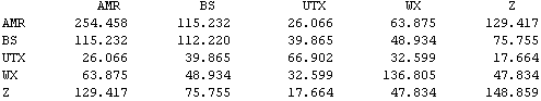
We will use these labels several times.
In[40]:=(label1 = "Markowitz Efficient Frontier";
label2 = {"Portfolio Variance", "Portfolio Mean"};
label3 = {"Portfolio Standard Deviation",
"Portfolio Mean"}; )
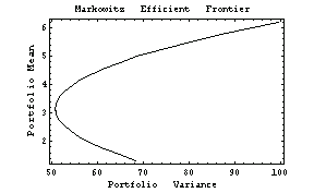
The efficient frontier is a parabola in the variance-mean plane.
In[41]:=ParametricPlot[Evaluate[EfficientFrontier[mean1, cov1, x]], {x, -.1, 1}, PlotLabel -> label1, FrameLabel -> label2];
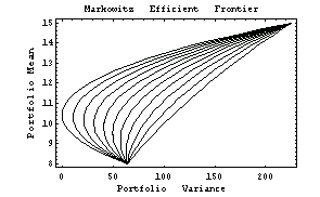
We can evaluate the risk of a portfolio with the functions PortfolioMean and PortfolioVariance.
Suppose our portfolio consists of two assets with mean returns of 8% and 15%.
In[42]:=mean2 = {8., 15.}
Out[42]=
Suppose we know the variances but not the correlation coefficient rho. The covariance matrix depends on rho.
In[43]:=cov2[rho_] = {{8.^2, 8. 15. rho}, {8. 15. rho, 15.^2}}
Out[43]=
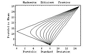
We find the Markowitz efficient frontier for different values of rho. Since we have only two assets it is more instructive to use PortfolioMean and PortfolioVariance than EfficientFrontier.
In[44]:=ParametricPlot[Evaluate[Table[{PortfolioVariance[
{x, 1-x}, cov2[rho]], PortfolioMean[{x, 1-x},
mean2]}, {rho, -1, 1, .2}]], {x, 0, 1},
PlotLabel -> label1, FrameLabel -> label2];
Sometimes the portfolio's standard deviation is used instead of the variance.
In[45]:=ParametricPlot[Evaluate[Table[
{Sqrt[PortfolioVariance[{x, 1-x}, cov2[rho]]],
PortfolioMean[{x, 1-x}, mean2]},
{rho, -1, 1, .2}]], {x, 0, 1},
PlotLabel -> label1, FrameLabel -> label3];
Betas and Security-Market Line
The Capital Asset Pricing Model (CAPM) is an equilibrium model of capital markets. The model's main conclusion is that the equilibrium relation between risk and return is given by the Security-Market Line
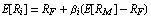
where  is the return on asset is the return on asset  and and  is the risk-free rate. is the risk-free rate.
We open a stream to the file stocks2.ret containing the returns of stocks.
In[46]:=stream = OpenRead[ToFileName[{"Finance","Data"}, "stocks2.ret"]];
We read in the number of assets.
In[47]:=n = Read[stream, Number]
Out[47]=
We read in the tickers.
In[48]:=tickers = Rest[Read[stream, Table[Word, {n+1}],
RecordSeparators -> {"\n", " ", "\t"}]]
Out[48]=
We read the rest of the data.
In[49]:=aux = Transpose[Partition[
ReadList[stream, Number], n+1]];
Finally we close the stream.
In[50]:=Close[stream];
We define lists of the months and returns of stocks.
In[51]:={months, returns} = {First[aux], Transpose[Rest[aux]]};
We will use the Standard & Poor 500 index as a model of the whole market. The file SP500.idx contains the values of the index for the same periods as the stocks in the file stocks2.ret. We have to compute the returns for this index.
We read in the dates and the values of the index.
In[52]:=idx = ReadList[ToFileName[{"Finance", "Data"}, "SP500.idx"],
{Number, Number}]
Out[52]=
This creates a list of index values only.
In[53]:=aux = Transpose[idx][[2]]
Out[53]=
We compute the returns for the Standard & Poor 500 index. We are assuming that they are good estimates for the returns of the whole market.
In[54]:=ret[SP500] ^= 100 (Rest[aux]/Drop[aux, -1] - 1)
Out[54]=
This creates a function ret that takes a stock ticker as an argument and gives the list of returns for that stock.
In[55]:=MapThread[ (ret[#1] ^= #2)&,
{ToExpression[tickers], Transpose[returns]}];
Here is the list of returns for AMR.
In[56]:=ret[AMR]
Out[56]=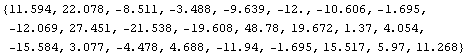
The built-in function Fit returns the formula for the regression line.
In[57]:=regressionLine[x_] = Fit[Transpose[{ret[SP500],
ret[AMR]}], {1, x}, x]
Out[57]=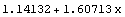
This defines a function that computes the beta of a given asset.
In[58]:=AssetBeta[marketreturns_List, assetreturns_List] :=
CoefficientList[Fit[Transpose[{marketreturns,
assetreturns}], {1, x}, x], x][[2]]
Here is the calculation of the beta for the AMR stock.
In[59]:=AssetBeta[ret[SP500], ret[AMR]]
Out[59]=
To perform a more sophisticated statistical analysis, load the standard statistics package.
In[60]:=Needs["Statistics`LinearRegression`"]
You can use the function Regress for linear regression analysis.
In[61]:=Regress[Transpose[{ret[SP500], ret[AMR]}], {1, x}, x]
Out[61]=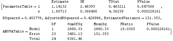
This explains the function.
In[62]:=?Regress
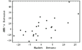
This is the graph of AMR's returns.
In[63]:=g1 = ListPlot[Transpose[{ret[SP500], ret[AMR]}],
PlotStyle -> PointSize[0.02],
PlotJoined->False,
FrameLabel -> {"Market Returns", "AMR's Returns"}];
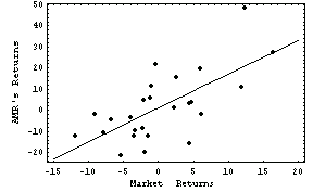
We generate a plot of the regression line, suppressing its display by setting the option DisplayFunction to Identity.
In[64]:=g2 = Plot[regressionLine[x], {x, -15, 20},
DisplayFunction -> Identity];
Now we display the data together with the regression line.
In[65]:=Show[g1, g2, DisplayFunction -> $DisplayFunction];
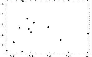
To compute the Security-Market Line we need the vector of average returns and the betas for all the stocks.
In[66]:=means = MeanVector[returns]
Out[66]=
In[67]:=betas = Map[ AssetBeta[ret[#], ret[SP500]]&,
ToExpression[tickers]]
Out[67]=
This is the regression data.
In[68]:=data1 = Transpose[{betas, means}]
Out[68]=
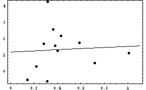
Here is the plot of the average returns versus the betas.
In[69]:=g3 = ListPlot[data1, PlotStyle -> PointSize[.02]];
This is the equation of the Security-Market Line.
In[70]:=securityMarketLine[x_] = Fit[data1, {1, x}, x]
Out[70]=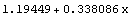
We generate a plot of the regression line, again suppressing its display.
In[71]:=g4 = Plot[securityMarketLine[x], {x, .0, 1.1},
DisplayFunction -> Identity];
Now we display the data together with the regression line.
In[72]:=Show[g3, g4, DisplayFunction -> $DisplayFunction];
Moving Averages
Some traders identify buy-sell opportunities by analyzing the moving averages of finance series.
First we load prices of IBM stock.
In[73]:=prices[IBM] ^= Last[Transpose[
ReadList[ToFileName[{"Finance", "Data"}, "IBM.prc"],
{Number, Number}]]];
The function MovingAverage is defined in the package Statistics`MovingAverage`. We compute the 15-day moving average for the last 1000 days.
In[74]:=
In[75]:=mavg[15] = Take[MovingAverage[prices[IBM], 15], -1000];
Here we compute the 75-day moving average for the last 1000 days.
In[76]:=mavg[75] = Take[MovingAverage[prices[IBM], 75], -1000];
We create the graph of the 15-day moving average.
In[77]:=g[15] = ListPlot[mavg[15],
PlotJoined -> True, DisplayFunction -> Identity];
We create the graph of the 75-day moving average.
In[78]:=g[75] = ListPlot[mavg[75],
PlotJoined -> True, DisplayFunction -> Identity];
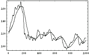
The intersection points of the moving averages identify trading opportunities.
In[79]:=Show[{g[15], g[75]}, DisplayFunction -> $DisplayFunction];
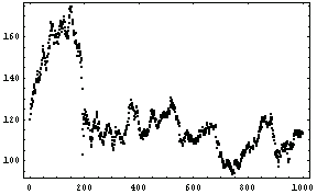
We create the graph of the prices.
In[80]:=g[0] = ListPlot[Take[prices[IBM], -1000]];
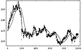
Finally we display all three graphs together.
In[81]:=Show[{g[0], g[15], g[75]},
DisplayFunction -> $DisplayFunction];
|