|
Getting Started
About the Package
You can solve many kinds of mathematical problems with the standard version of Mathematica. However, financial experts need functions that are not built into Mathematica or included in any of the standard packages. The Finance Pack is designed to provide an introduction to using Mathematica in financial analysis. Some very elementary examples of Mathematica programming are presented in order to stimulate users to write their own financial programs and packages. To use the Finance Pack, basic familiarity with the Mathematica kernel and the notebook front end is assumed. The Finance Pack has three components: packages, data files, and notebooks.
Packages are the main part of the Finance Pack. They are files written in the Mathematica language that contain definitions that extend the system. You may modify or use them in your own algorithms. They are just like packages from the standard Mathematica distribution. The notebook front end is not required to use them.
The data files are needed to reproduce some of the examples from this guide.
Mathematica notebooks are interactive documents combining Mathematica input, output, text, and graphics. For more information see the user's guide for your Mathematica front end. The notebooks provided with the Finance Pack are the on-line version of this document.
Installing the Finance Pack
The Finance Pack is easy to install. Make sure you have Mathematica installed on your computer and follow the steps described on the installation card. The installation program will (if needed) create a directory for the Mathematica applications and subdirectories for the Finance Pack. Then it will copy what you choose from the distribution media into the right directories. Just follow the directions on the screen.
Loading the Finance Pack
After starting a Mathematica session we load the package.
Here is the most convenient way to load the package.
In[1]:=<< Finance`
Now all the functions from the Finance Pack are available. Any subpackages that are needed will be loaded automatically.
The Finance Pack includes the following subpackages:
Finance`Calendar`
Finance`InterestRates`
Finance`Bonds`
Finance`Options`
Finance`Examples`
Finance`Common`
Finance`Kernel`init`
To instruct Mathematica to load an individual subpackage, use the command << filename or Get["filename"] or Needs["context"]. If the package directory is in the current search path, then Mathematica will find the package and load it. You can also include the full path name of the package. In that case Mathematica will look only in the place you have specified.
This loads the subpackage Finance`Bonds`.
In[1]:=<< Finance`Bonds`
The Concept of Finance Objects
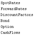
The functions used in finance are mostly polymorphic; that is, the way they work depends on the type of arguments they use. They might also have a variable number of arguments. Mathematica can handle either situation easily and correctly. The package implements the concept of a finance object.
In[1]:=<< Finance`
These are the available classes of finance objects.
In[2]:=?FinanceClasses

This is the general way to define a finance object  . .
f = Class[description, options]
The description is a list of parameters necessary to define an object. It is important to keep them in the right order. Setting the second argument modifies the behavior of the functions that act on the object. Don't confuse options with the finance object Option.
This defines the finance object xyzft. Here we use only the first argument.
In[3]:=xyzft = Option[{"Put", XYZ, 40, {12, 20, 1992}}]
Out[3]=
Here is another finance object, bond3, defined using the option CountDayBasis -> "30/360".
In[4]:=bond3 = Bond[{.10, {9, 15, 1993}, 1000 USDollar, 2},
CountDayBasis -> "30/360"]
Out[4]=
We will discuss how to create and use finance objects in detail in the following sections.
Names
The convention that has been adopted for built-in Mathematica objects is to use full English names with the first letter of each word comprising the name capitalized, for example, PresentValue, YieldToMaturity, etc. You may prefer to use your own naming system.
Here is an example of a present value calculation.
In[5]:=PresentValue[1000 USDollar, 7.26 Percent, 1, 2]
Out[5]=
Here we define the alias PV for PresentValue.
In[6]:=PV = PresentValue
Out[6]=
PV works in exactly the same way as PresentValue. Note that using short names and aliases instead of full names sometimes leads to confusion.
In[7]:=PV[1000 USDollar, 7.26 Percent, 1, 2]
Out[7]=
You can create a file defining your aliases and read it in at the beginning of your Mathematica session or you can define aliases in the file init.m so that they will be available for each Mathematica session.
|