2.5 Fuzzy Logic Control

2.5.1 Introduction

In this notebook, we look at how to design a fuzzy logic control strategy to back a truck up to a loading dock.

The goal of the controller is to come up with a steering strategy to back-up a truck so that it arrives perpendicular to a dock. The truck may start at any initial position and orientation in the parking lot. To model this scenario, we assume our parking lot is a graph that is 100 units wide and 100 units tall. Our loading dock is located at the top-center of the graph at position {50, 100}. Our controller decides what steering angle is needed at each stage to back the truck up correctly. We limit the steering angle to be between -30 and 30 degrees.

To implement our fuzzy logic controller, we use many of the commands from Fuzzy Logic as well as a few additional routines to model the truck [Freeman 1994].

This loads the package.

In[1]:=

2.5.2 Defining Input Membership Functions

Truck Position

Set Universal Space

One of the first questions to ask when designing a fuzzy logic controller is the following: What are my inputs and outputs? Once this question is answered, the next item to address is the range of the inputs and outputs. When talking about fuzzy sets, this range is referred to as the universal space.

In our example, the first input we use is the truck's x-position on the graph. Since we decided on a parking lot 100 units wide, we need a universal space that ranges from 0 to 100. To simplify the later construction of our membership functions, we change the default universal space now to be the desired range, 0 to 100, with the following command.

In[2]:=

Define Linguistic Variables

We next need to decide on the number and shape of the membership functions to use. There is no optimal solution for choosing membership functions, only guidelines. We do not worry about that here, we simply follow the example used by Kosko [Kosko 1992].

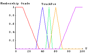
We use the FuzzyTrapezoid function to construct our membership functions. The names of our fuzzy sets have the following linguistic meanings: LE-Left, LC-LeftCenter, CE-Center, RC-RightCenter, and RI-Right. These variables are used to describe the truck's x-position on the graph. We collect all the membership functions together under the heading TruckPos, which is the first input to our controller.

In[3]:=

In[8]:=

Plot the Membership Functions

Next, we plot the membership functions for our first input with the FuzzyPlot function. The PlotJoined option is set to True to produce the line graph shown.

In[9]:=

Truck Angle

Set Universal Space

The second input is the truck's orientation or the angle between a line down the center of the truck and a line horizontal to the parking lot. For this input, the universal space ranges from -90 degree, where the back of the truck is facing away from the dock, to 270 degrees, where it is again facing away. The truck angle should end up near 90 degrees, which indicates that the back is facing the dock and the truck is perpendicular to the dock. For angles between -90 and 90 degrees, the back of the truck will be facing toward the right of the graph, and for angles between 90 and 270 degrees, the back of the truck will face the left side of the graph.

We set the universal space for our second input just as we did for our first input.

In[10]:=

Define Linguistic Variables

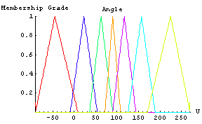
We again use Kosko's membership functions [Kosko 1992] for this input. The linguistic variables have the following meanings: RB-Right Below, RU-Right Upper, RV-Right Vertical, VE-Vertical, LV-Left Vertical, LU-Left Upper, and LB-Left Below. We group all of the membership functions under the name Angle, which is the second input to our controller.

In[11]:=

In[18]:=

Plot Membership Functions

Here is a plot of the second input's membership functions.

In[19]:=

2.5.3 Defining Output Membership Functions

Set Universal Space

The output of our controller is a steering angle limited to the range -30 to 30 degrees. This then is the universal space we need for our output membership functions.

In[20]:=

Defining Linguistic Variables

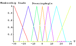
We again use the membership function definitions from the Kosko book [Kosko 1992] to define our output membership functions. This time we name our membership functions : NB-Negative Big, NM-Negative Medium, NS-Negative Small, ZE-Zero, PS-Positive Small, PM-Positive Medium, PB-Positive Big. These names are used frequently in defining fuzzy logic controllers. We group all the output membership functions under the name SteeringAngle, which is our single output.

In[21]:=

In[28]:=

Plot Membership Functions

Here we see how our output membership functions looks.

In[29]:=

2.5.4 Defining Control Rules

The final item needed for a fuzzy logic controller is a set of rules or a rule base. Typically rules for fuzzy logic controllers appear in if-then form. Our fuzzy inference system accepts rules as a list of triplets. The first two item in each triplet are the input conditions and the third item is the output condition.

This list represents rules of the form: if input1 = #1 and input2 = #2, then output = #3. For example, looking at the following control rules, the first rule, {LE,RB,PS}, represents the linguistic rule: if TruckPos is LE (Left) and Angle is RB (Right Below), then SteeringAngle should be PS (Positive Small). The rules are formed with linguistic terms, which follow human intuition.

In[30]:=

2.5.5 Simulation Functions

This section contains functions that will allow us to simulate the truck backing. This first function is essentially the fuzzy logic controller. The two inputs to this function, phi and x, represent the two inputs to the controller, the angle and truck position. The function will return a crisp output that is the controller's recommended steering angle.

In[31]:=

These next two functions are for modeling the truck-backing. They contain functions that model the movement of the truck and draw the parking lot and truck graphics. These functions are from a Mathematica Journal article by James Freeman [Freeman 1994].

In[32]:=

In[33]:=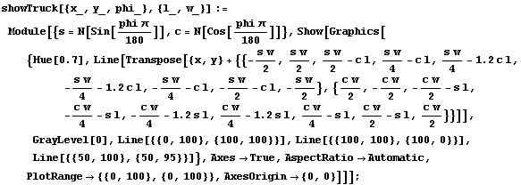

2.5.6 Test Run 1

Run Simulation

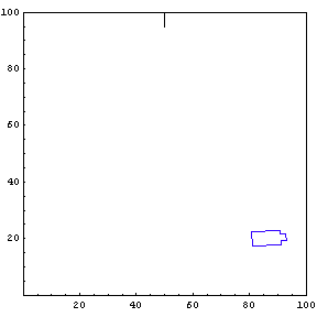
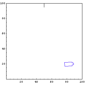
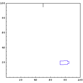
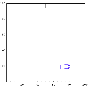
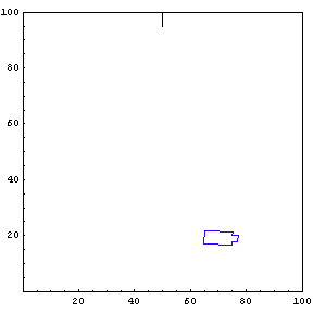
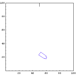
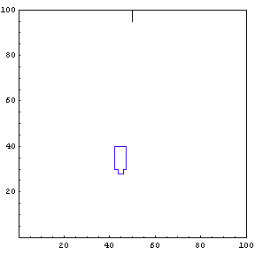
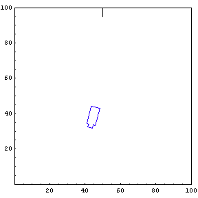
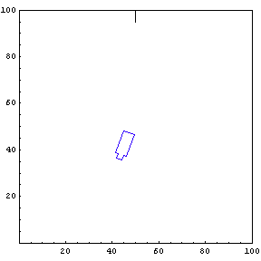
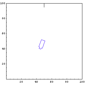
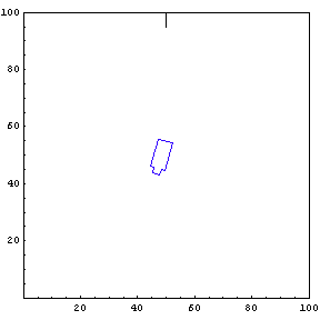
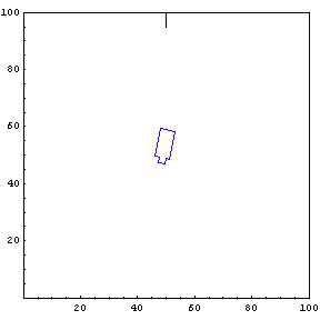
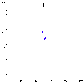
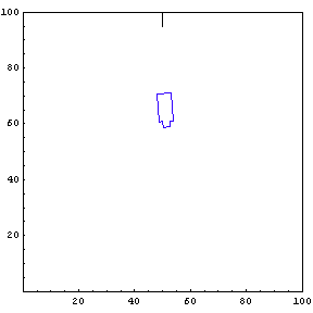
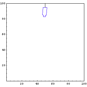
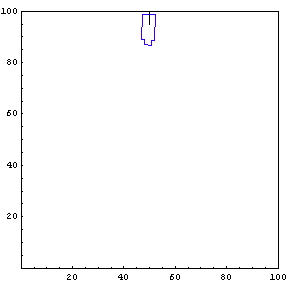
We provide the function simulateTruck with an initial x-position, y-position, and truck angle. For the first simulation, we start the truck at position {85, 20} with an initial angle of 190 degrees.

In[34]:=

Model Results

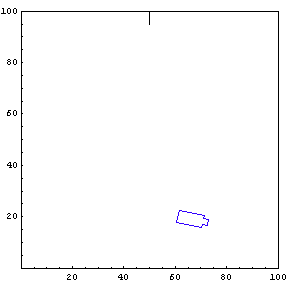
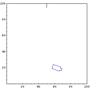
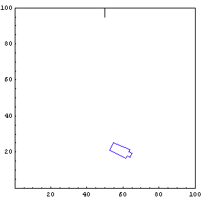
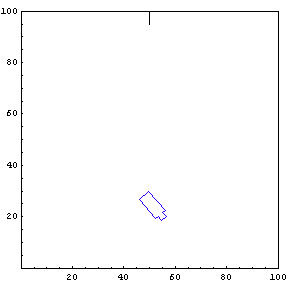
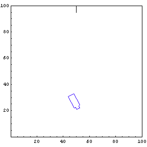
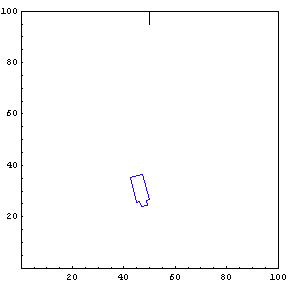
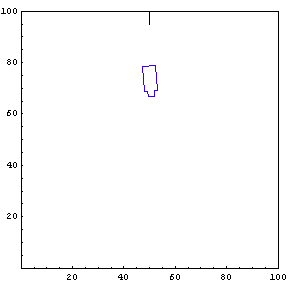
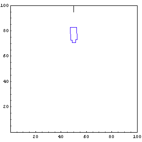
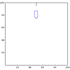
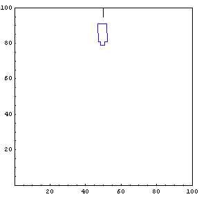
The function below will draw a graph showing the location and angle of the truck in the parking lot. To see an animation of the truck backing, click the cell bracket containing all of the truck graphics; this will highlight the bracket. Now select Animate Selected Graphics from the Graph pull down menu. This will cause the truck to appear to move in one of the graphs. The buttons that appear at the bottom border during animations can be used to control the speed and direction of the animation. To stop the animation click anywhere in the notebook.

In[35]:=

Show Complete Trajectory

The complete trajectory of the truck can be seen using the Show command.

In[36]:=

2.5.7 Test Run 2

Run Simulation

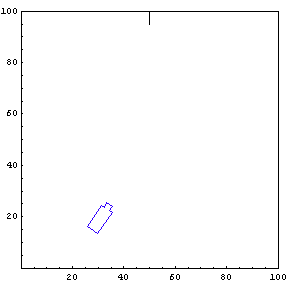
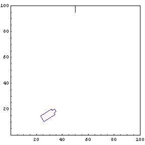
We can run another simulation from a different starting position and angle. You can test this program with your own initial values for x, y, and phi. The controller should work if there is enough room from any position and angle.

In[37]:=

Model Results

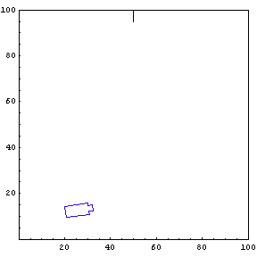
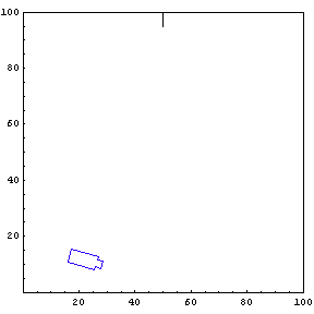
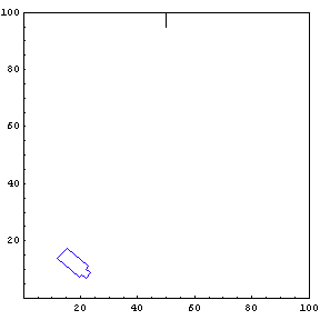
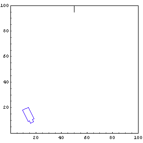
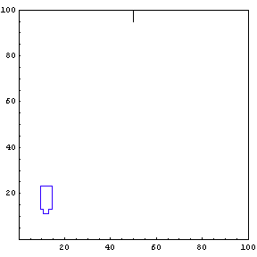
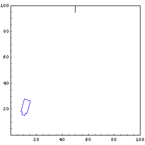
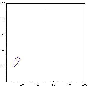
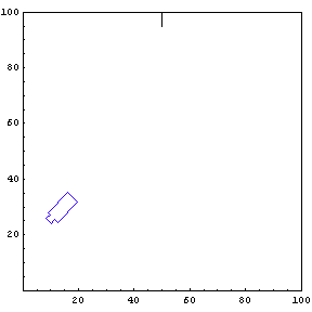
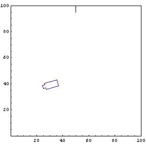
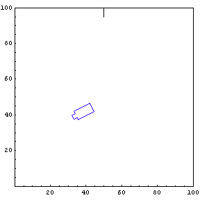
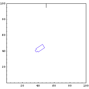
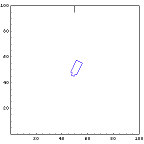
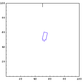
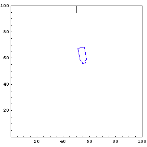
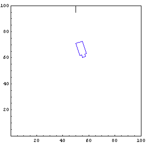
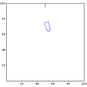
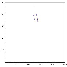
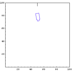
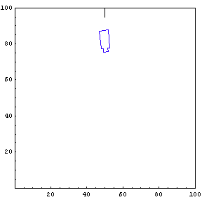
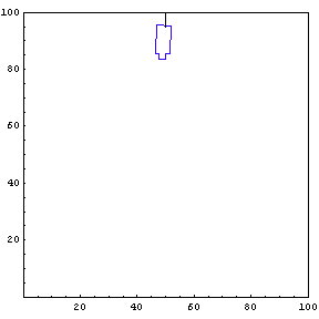
We again model the results. You can again animate the graphic cells in this section using the animation option.

In[38]:=

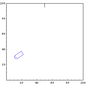
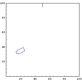
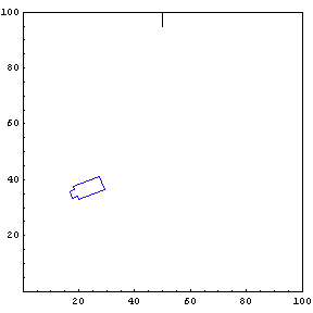
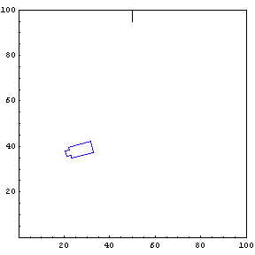
Complete Trajectory

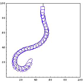
Again, we show the complete trajectory of our second test run.

In[39]:=

2.5.8 Control Surface

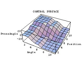
A convenient way to examine a two-input/one-output control strategy is to look at a control surface. This is a 3D graph in which the inputs form the base of the graph, and the output is represented by the height of the graph above each input pair. We have constructed such a surface here.

In[40]:=

In[41]:=

References

J. A. Freeman, Fuzzy systems for control applications: the truck backer-upper, The Mathematica Journal, vol. 4, pp. 64-69, 1994.

B. Kosko, Neural Networks and Fuzzy Systems: A Dynamical Systems Approach to Machine Intelligence, Prentice Hall, Englewood Cliffs, NJ, 1992.