|
3.9.6 TransientPlot
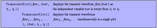
Command structure of TransientPlot.
TransientPlot displays one or several transient waveforms in a single plot, where the signal values are usually plotted versus time.
Note that TransientPlot has attribute HoldAll.
Additionally, TransientPlot supports the multi-dimensional data format of Analog Insydes described in Section 3.7.1, which consists of lists of rules, where the variables are assigned InterpolatingFunction objects. Therefore, call TransientPlot where the first argument is compatible to the return value of the numerical solver functions NDAESolve and NDSolve, or the data interface function ReadSimulationData:
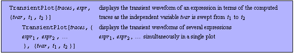
Displaying numerical data with TransientPlot.
TransientPlot inherits most of its options from Plot and GraphicsArray. Both the options which are specific to TransientPlot as well as the inherited options can be set with SetOptions[TransientPlot, opts].
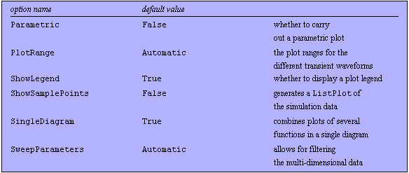
Options for TransientPlot.
See also: NDSolve, NDAESolve, ReadSimulationData.
Options Description
A detailed description of all options that are specific to TransientPlot or are used in a non-standard way is given below in alphabetical order:
Parametric
Changing the default setting from False to True allows for carrying out parametric plots of transient waveforms. Therefore, specify a list of two expressions, where the first one refers to the  -axis and the second to the -axis and the second to the  -axis. The expressions are automatically added as labels to the -axis. The expressions are automatically added as labels to the  and and  -axes. -axes.
Please note that this option also supports the multi-dimensional data format.
PlotRange
The usage of the option PlotRange is different as compared to Plot. The PlotRange of each transient waveform can be separately modified for the setting SingleDiagram -> False. The default setting is PlotRange -> Automatic. Possible option values are as follows:

Values for the PlotRange option.
ShowLegend
The option ShowLegend allows for displaying a plot legend. The default setting is ShowLegend -> True.
ShowSamplePoints
Changing the default setting from False to True allows for generating a ListPlot of the simulation data.
Please note that this option also supports the multi-dimensional data format.
SingleDiagram
The option SingleDiagram combines plots of several transient waveforms in a single diagram. Changing the default setting from True to False produces a GraphicsArray of separately plotted transient waveforms.
Please note that this option also supports the multi-dimensional data format.
SweepParameters
The option SweepParameters allows for filtering the multi-dimensional data. The default setting is SweepParameters -> Automatic. Possible option values are as follows:

Values for the SweepParameters option.
Examples
Load Analog Insydes.
In[1]:= <<AnalogInsydes`
Plot two sinusoidal functions.
In[2]:= S[T_] := Sin[10.T];
TransientPlot[{S[T], 2 S[T-1]}, {T, 0, 1}]
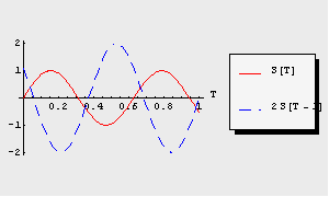
Out[3]= 
In the following, the transient solution of the diode rectifier circuit shown below is plotted using TransientPlot.
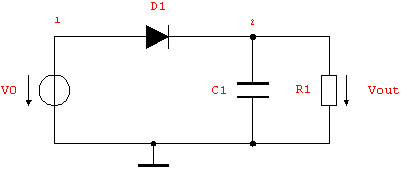
Define netlist description of a simple diode rectifier circuit.
In[3]:= rectifier =
Circuit[
Netlist[
{V0, {1, 0}, Symbolic -> V0,
Value -> 2. Sin[10^6 Time]},
{R1, {2, 0}, Symbolic -> R1, Value -> 100.},
{C1, {2, 0}, Symbolic -> C1, Value -> 1.*^-7},
{D1, {1 -> A, 2 -> C},
Model -> "Diode", Selector -> "Spice"}
]
]
Out[4]= 
Set up system of symbolic time-domain equations.
In[4]:= rectifiereqs = CircuitEquations[rectifier,
AnalysisMode -> Transient, ElementValues -> Symbolic]
Out[5]= 
Perform numerical transient analysis.
In[5]:= tran = NDAESolve[rectifiereqs, {t, 0., 2.*^-5}]
Out[6]= 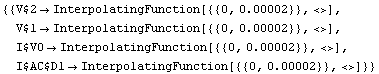
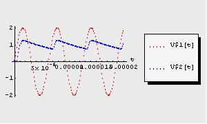
Display the simulation result with TransientPlot for the variables V$1[t] and V$2[t].
In[6]:= TransientPlot[tran, {V$1[t], V$2[t]}, {t, 0., 2.*^-5},
Axes -> False, Frame -> True, GridLines -> Automatic]
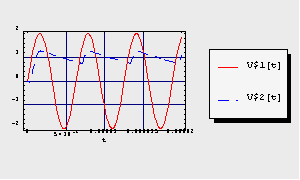
Out[7]= 
View signals separately.
In[7]:= Vd[t_] := V$1[t] - V$2[t];
TransientPlot[tran, {Vd[t], V$2[t]}, {t, 0., 2.*^-5},
PlotRange -> {{-4., 2.}, {0., 1.5}},
SingleDiagram -> False]
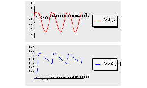
Out[9]= 
Display the simulation data.
In[8]:= TransientPlot[tran, {V$1[t], V$2[t]}, {t, 0., 2.*^-5},
ShowSamplePoints -> True]
Out[10]= 
Generate a parametric plot.
In[9]:= TransientPlot[tran, {V$1[t], V$2[t]},
{t, 2.*^-6, 2.*^-5}, Parametric -> True]
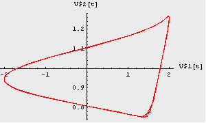
Out[11]= 
Perform parametric transient analysis.
In[10]:= paramtran = NDAESolve[rectifiereqs, {t, 0., 2.*^-5},
{R1, Table[10^i, {i, 0, 3}]}]
Out[12]= 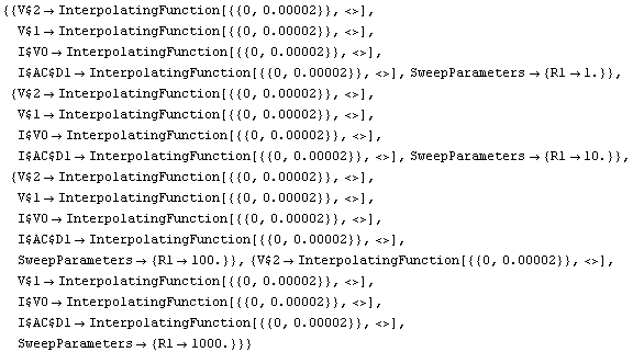
Display the multi-dimensional simulation result: show all traces of the parameter sweep.
In[11]:= TransientPlot[paramtran, {V$2[t]}, {t, 0., 2.*^-5}]
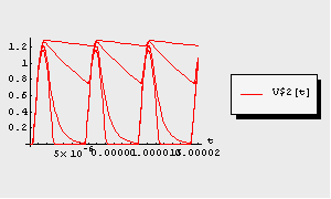
Out[13]= 
Filter the multi-dimensional data: display only the trace corresponding to the parameter value R1=1.
In[12]:= TransientPlot[paramtran, {V$2[t]}, {t, 0., 2.*^-5},
SweepParameters -> {R1 -> 1.}]

Out[14]= 
|