Cams & Followers

Example Mechanism for MechanicalSystems Cam Constraints

by Robert Beretta

Cam Animation

Discussion

Cam-Follower Function

This sample notebook analyzes the motion of several cam-follower mechanisms. Each mechanism consists of a simple rotating cam and a rocker type follower. The use of Modeler2D's four cam constraints is demonstrated, as well as different techniques for specifying cam profiles.

Cam-Follower Model

The cam-follower mechanism consists of three bodies.
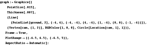
1. Ground    (black)
2. Cam    (red)
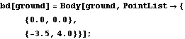
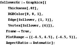
3. Follower    (blue)

Kinematic Model

Preparation

The Modeler2D package is loaded into Mathematica with the Needs command.

The following symbols are used to reference each of the bodies in the cam-follower model throughout the analysis.

The following is done simply to prevent the generation of unwanted spelling errors.

Body Definitions

Ground

Two points are defined on the ground (body 1).
P1. The cam axis (at the local origin).
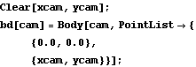
P2. The pivot point of the follower.

Cam

Two points are defined on the cam (body 2).
P1. The rotational axis of the cam.
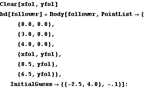
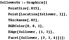
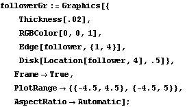
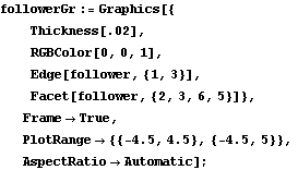
P2. The point of contact between the cam and the follower, on the cam. The coordinates of this point are not constant; rather the coordinates are both defined as functions of an independent variable. Thus the cam's profile is the locus of this point as the independent variable is varied.

Follower

Five points are defined on the follower (body 3). These points are not all used by the same mechanism; they will be used when the model is changed to accommodate different cam constraints.
P1. The rotational axis of the follower.
P2. and P3. The points used for the graphic image.
P4. The point of contact between the cam and the follower, on the follower.
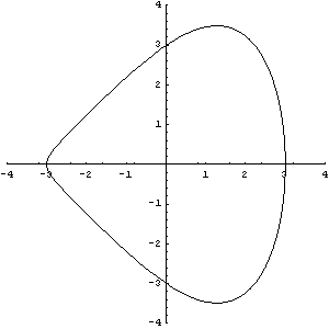
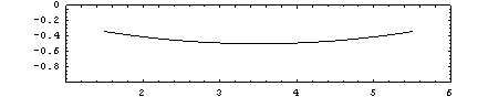
P5. and P6. Two points defining a flat surface of contact (for CamToLine1[]).

Build bodies

The data contained in each of the body objects is entered into the current model with the SetBodies command.

Cam and Follower Profiles

Here are the parametric equations defining the locus of the cam profile.

For the first demo the contact point is constant on the follower, so point 4 is given a constant value. Here are initial constants for what will be the follower profile in future models.

ParametricPlot shows the profile in the base position. The body 2 local origin is the plot origin.

Constraint Definitions

Standard constraints

Three standard constraints and one cam constraint are required to model the cam-follower mechanism.

1. A revolute joint to place the cam axis.

2. A driving constraint to control the rotational position of the cam.

3. A revolute joint to place the pivot point of the follower on the ground.

CamToPoint1

The numerical value of the variable that controls the contact point on the surface of the cam must be found along with all the other dependent variables. This variable is added to the model automatically by the cam constraint object.

It should be noted, however, that each cam surface adds one degree of freedom to the model and each cam constraint controls two degrees of freedom. Thus, cam constraints are applied as if they are one degree of freedom constraints, though they actually constrain two degree of freedom (or more).

Five degrees of freedom are constrained in the model so far, and the last mechanical degree of freedom plus the extra degree of freedom associated with the cam are constrained with a CamToPoint1 constraint.

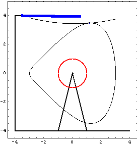
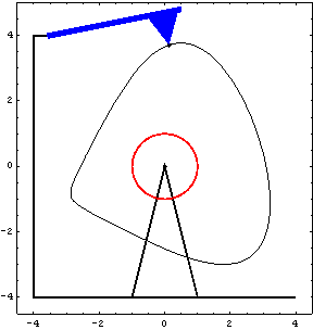
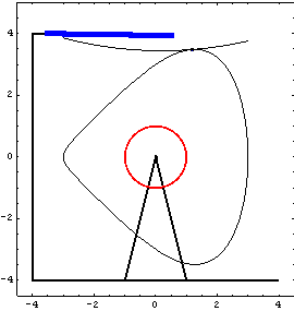
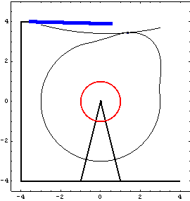
SetConstraints incorporates the constraint objects into the current model.

Running the Model

CheckSystem tests the model for redundant constraints, undefined variables, and so forth.

Now we solve the model with time set to 0.05.

Graphics

Here is the graphic image of the ground and the cam.

Here is the graphic image of the follower.

The cam profiles are generated using the CamPlot graphics function, which draws the same profile as was plotted earlier with ParametricPlot and locates the profile correctly in 2D space.

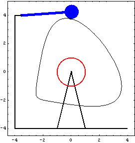
Other Cam Constraints

CamToCircle1

CamToCircle1 models a cam follower that has a finite radius, instead of an infinitesimal radius like CamToPoint1.

The first three constraints in the following set were defined previously.

Graphics

CamToLine1

CamToLine1 models a flat cam follower.

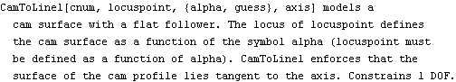
The first three constraints in the following set were defined previously.

Graphics

CamToCam1

CamToCam1 models two cammed surfaces working against each other.

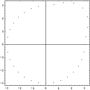
To use CamToCam1 another cam profile is defined on the follower. This profile is the locus of point 3 on the follower.

Here is a plot of the follower profile.

The first three constraints in the following set were defined previously.

Graphics

Animation

The following input generates the 24 animation frames at the beginning of this notebook.

The following cell must be made evaluatable to generate the animation.

Mapped Cams

Cam Profile

Most real cam surfaces cannot be easily described by analytic functions, like the example cam surface used previously. Cams are more generally mapped numerically as a series of 2D points that are interpolated to make a smooth surface.

Mathematica's InterpolatingFunction provides a convenient way to model cams in this manner. The two parametric equations that were used to describe the x and y coordinates of the profile, as functions of alpha, are replaced by two InterpolatingFunction objects.

First, data is entered as a list of 8 points to describe the first 90° of the cam.

The last 270 degrees of the cam profile is simply a circle, so the next 25 points are generated automatically.

Two interpolating functions must be generated--one for x and one for y.

Note that the value of the contact point parameter, alpha, nows runs from 1 to 33 as the contact point travels around the cam, instead of from 0 to 2. While this is somewhat nonintuitive, it works just fine.

Note also the the value of alpha cannot be outside the range of the InterpolatingFunction, and if Modeler2D's solution block attempts to take it there, an error will result.

Running SetConstraints can take quite a while because the InterpolatingFunction objects must be differentiated with respect to alpha, which requires the generation of new InterpolatingFunction objects.

Graphics

You may have noticed that the model ran very slowly with the mapped cam profile. This is because of the very large number of calculations being done to evaluate the InterpolatingFunction objects. In general, if it is possible to describe the cam profile with an analytic function; do so. Mapped cam profiles also have trouble converging at times; when this happens, the ZeroTest option should be changed to make the convergence test easier to pass.

End