7.4.2 2D Example Mechanism To demonstrate the use of Mech's StageSwitch function, a 2D model is developed that is subject to a variable applied load. The model is a simple piston-pump that has a nonlinear compression function applied to the piston.
The input to the model is to rotate the crankshaft. The pressure on the piston increases slowly but nonlinearly until near the end of its stroke, at which time the pressure decreases very rapidly back to zero. The pressure then remains at zero through the return stroke of the piston. Here is the 2D piston-pump graphic.
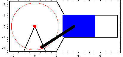
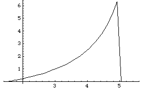
ConstraintsFour constraints, one of which is a driving constraint, are required to model the piston-pump. Body objects are not defined for this model. The coordinates of the local points are simply entered directly in the point and axis objects in the constraints. A Revolute2 constraint constrains the center of the crank to be coincident with the global origin.A RelativeDistance1 constraint models the connecting rod by placing the piston a constant distance from an eccentric point on the crank.A Translate2 constraint models the piston and cylinder by constraining the piston to translate along a horizontal line on the ground body.A RotationLock1 constraint is the driving constraint that makes the crank angle a function of time.Names are defined for each of the bodies in the model. Here are the constraint objects for the model. Here is a reasonable initial guess for the piston. Loads Only one load is applied to the piston-pump model, but this one load will be a two-stage StageSwitch load. Since the piston is initially at the top of its stroke and proceeds toward the bottom, there is no load on the piston for the first half turn of crank rotation. The two segments of the StageSwitch load are defined as follows. Stage one is a Force on the piston that rises from zero at bottom-dead-center to seven units when the X coordinate of the piston is equal to 5.0.Stage two is a Force on the piston that falls from seven units back to zero as the X coordinate of the piston goes from 5.0 to 5.5.Here are the two forces on the piston. The StageSwitch load must switch between f1 and f2 at the proper time. This is done by testing the value of the X coordinate of the piston X3 and the angular coordinate of the crank  2. 2. Here is the StageSwitch load object for the pump.
Out[20]= |  |
The loads are incorporated into the model. Running the Model The loaded model can now be run with the Solution -> Static option for SolveMech. Note that all of the loads are zero at T = 0.1 because the force is turned off. Now run the model at T = 0.1.
Out[22]= |  |
Here is the piston-pump model at T = 0.1.
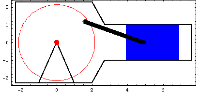
By creating a large table of solution points, plots can be made of various forces, moments, and reactions in the model using ListPlot. Here is a list of 81 solutions. The Loads function returns the total load on the piston.
Out[24]= |  |
The force on the piston can be plotted as a function of piston travel.
Out[25]= |  |
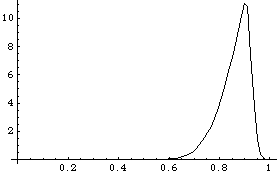
The reaction forces at the constraints can be found with the Reaction function. Constraint 4 is the RotationLock1 driving constraint, so its reaction is the moment applied to the crank. Constraint 1 is the Revolute2 constraint that positions the crank axis, so its reactions are the X and Y forces supporting the crank axis. Here is the moment required to rotate the crank.
Out[26]= |  |
Here is the reaction at the crank as a function of time.
Out[27]= |  |
Because ListPlot is not able to plot two lists simultaneously, Mathematica graphics primitives are used directly to plot the X and Y reactions. Here are the X and Y reaction forces at the crank axis as a function of time.
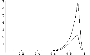
Out[28]= |  |
|