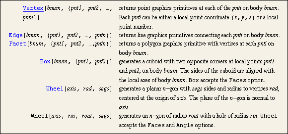
3.5 3D Mechanism ImagesThis section demonstrates the special Modeler3D graphics functions that are used to generate the mechanism images throughout this document. Modeler3D graphics functions return graphics primitives that are given as arguments to the Mathematica Graphics function and displayed with the Show command, just like the built-in Mathematica graphics primitives.
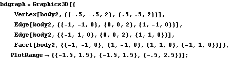
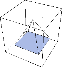
The primary utility of the Modeler3D graphics functions is that they take their arguments in the form of local coordinates and automatically convert them to global. Thus, it is possible to create the image of a mechanism part using the same techniques as would be used with built-in Mathematica graphics primitives, and then have the part be positioned properly with respect to the other parts of the mechanism automatically, as specified by a Modeler3D solution rule. 3.5.1 Graphics FunctionsThe elementary Modeler3D graphics functions closely parallel the built-in Mathematica graphics primitives. Each graphics function generates Mathematica graphics primitives that represent points, lines, or polygons. The Modeler3D compound graphics functions generate more complex shapes, such as spheres and cylinders. Basic 3D graphics functions. More 3D graphics functions. Options for graphics functions. The Modeler3D Vertex, Edge, and Facet functions are analogous to the built-in Mathematica Point, Line, and Polygon graphics primitives. To demonstrate these functions, graphics objects are generated on body 2, which is named body2. This loads the Modeler3D package. Here is a pyramid with a filled floor. The coordinates of the graphic just created bdgraph are functions of the Modeler3D variables that locate body2: X2, Y2, Z2, Eo2, Ei2, Ej2, and Ek2. Therefore, these variables must be replaced with numeric values before trying to Show the graphic. Here is bdgraph located coincidentally with the local origin.
Out[5]= |  |
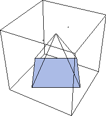
To show the pyramid in another orientation, a set of four Euler parameters are fabricated that represent the desired angular orientation. Normally, Modeler3D graphics functions are used in conjunction with a Modeler3D solution rule that contains the values of the Euler parameters needed, but in this case they are generated explicitly.
The pyramid is now rotated 0.5 radians about the global Z axis. The EulerParameters function returns the Euler parameters required for this rotation. These Euler parameters represent a rotation of 0.5 radians about the {0, 0, 1} axis.
Out[6]= |  |
Now the parameters are turned into rules for Eo2, Ei2, Ej2, and Ek2.
Out[7]= |  |
Here is bdgraph rotated 0.5 radians about the Z axis.
Out[8]= |  |
The Box function is analogous to the built-in Cuboid function, with the exception that the sides of the Box graphic are aligned with the local coordinate system on which the graphic is located, instead of being aligned with the global coordinate system.
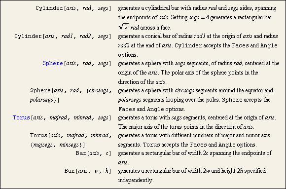
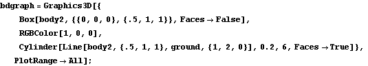
The Cylinder function generates a faceted cylinder or cone, with endpoints located at the two ends of a Modeler3D line object. The Faces option is used with Cylinder to show only an outline of the cylinder. Here is a Box graphic on body2 and a Cylinder graphic spanning from body2 to the ground. Here is the result.
Out[10]= |  |
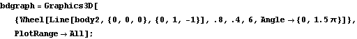
The Wheel function is used here to generate a part of an octagon with a hole in it. Note that the n-gon returned by Wheel is placed on the body that is referenced in the Point argument, and is located with that body as such. This generates a piece of an octagon on body2. Here is the result.
Out[12]= |  |
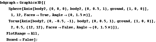
The Sphere and Torus functions are used here to generate a sphere and a torus. This generates a piece of a sphere and a torus on body2. Here is the result.
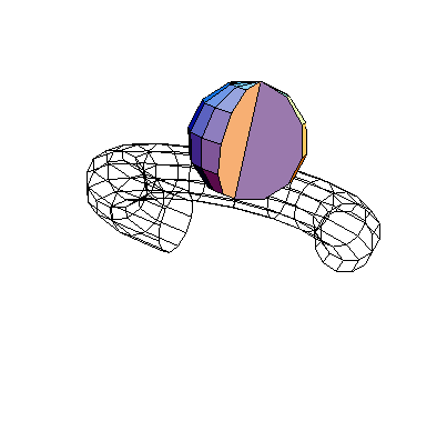
Out[14]= |  |
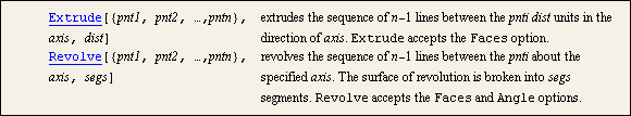
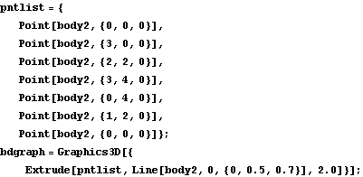
Functions to generate pseudo-solid objects. Extrude is used to generate a sequence of faces that are defined by sweeping a sequence of connected lines through 3D space. The following example takes six points on body2 that define an hourglass form and extrudes them at an oblique angle into a set of six facets forming a canted hourglass. Here are the points for an hourglass graphic. The graphic is shown shifted 2 units in the Y direction off of the global origin.
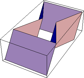
Out[17]= |  |
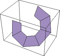
The same list of points can be revolved about an axis specified on body2. Here is a revolution of the hourglass graphic. Here is the result.
Out[19]= |  |
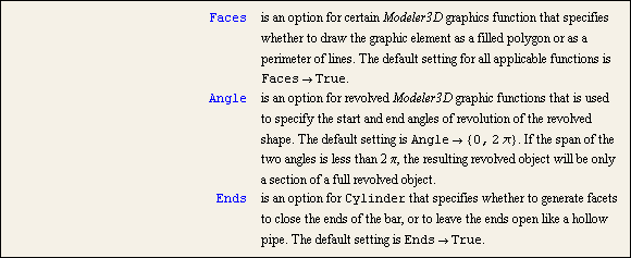
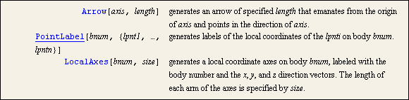
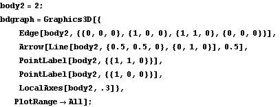
3.5.2 Annotation FunctionsThree graphics functions are provided by Modeler3D specifically for annotation. Graphics functions for annotation. PointLabel and LocalAxes can be used to conveniently label points and bodies. The following input generates a triangle placed on body 2, with two of the points labeled with their body numbers and local coordinates. This generates the triangle graphic. Here is the result.
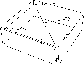
Out[22]= |  |
A function for plotting the locus of a moving point. The nested list of rules required by LocusPlot is of the form returned by SolveMech. 3.5.3 Example Mechanism GraphicsThe spatial slider-crank mechanism model that was developed in Section 3.2 is used to demonstrate the use of Modeler3D graphics functions to create an image of a mechanism model. Creating a complex mechanism image often requires more lines of Mathematica code than were used in the kinematic model of the mechanism. This is because of the terse nature of the data required to kinematically describe a mechanism. A kinematic model uses only a small number of points in space to define rotational and translational axes that tie the bodies together, while the mechanism image requires much more information about the shape of the bodies in the model.
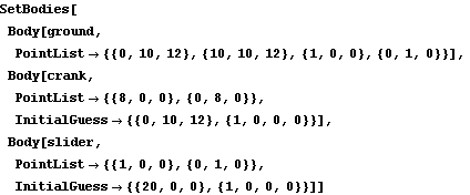
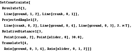
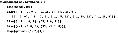
The spatial slider-crank model is redefined as follows in abbreviated form. See Section 3.2 for a full description of this mechanism model. Here is the complete definition of the slider-crank model. To demonstrate the use of the graphics functions the image of the slider-crank mechanism that is displayed in the preceding sections is built. These images are generated with a mix of Modeler3D graphics functions and built-in Mathematica graphics primitives. GroundThe ground body of the slider-crank mechanism was generated using mostly built-in Mathematica graphics primitives. The Modeler3D Edge function was used to generate a line on the crank axis referencing local points by their point numbers. Here is the ground body graphic. The text that was displayed with the ground body was generated entirely with the built-in Mathematica Text function, except for the axes at the global coordinate origin, generated with the Modeler3D LocalAxes function, and the use of the Location function to reference the global coordinates of local point numbers on the ground body. Here is the ground body annotation. Here is the result.
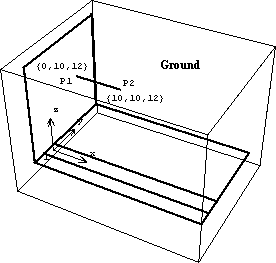
Out[30]= |  |
CrankThe crank graphic uses the Modeler3D Cylinder function to generate a very short cylinder. The cylinder is only one unit long because the line that defines its axis is one unit long, while the radius of the cylinder is ten units as specified. Here is the crank body graphic. The text that was displayed with the crank graphic also used the Location function to specify the global coordinates of the text so that the text moves with the crank. Here is the crank annotation. Because the coordinates of some of the elements in crankgraphic and cranktext are now functions of Modeler3D dependent variables, X2, Y2, and so on, a Modeler3D solution rule must be applied before they can be displayed. Note the use of SolveMech in the following input. The rules that are returned by SolveMech determine where the crank is located in 3D space. Here is the result.
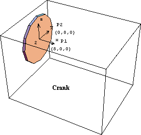
Out[33]= |  |
SliderThe slider graphic uses the Modeler3D Box function to generate the rectangular box form of the slider. Here is the slider graphic. Here is the slider annotation. Like the crank graphic, the coordinates in the slider graphic are functions of Modeler3D dependent variables. Thus, a solution rule must be applied to display the graphic. Show it.
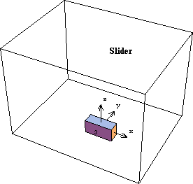
Out[36]= |  |
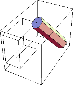
Connecting RodThe connecting rod graphic uses the Modeler3D Cylinder function again to generate a long, thin cylinder spanning from the crank to the slider. Here is the connecting rod graphic. Here is the connecting rod annotation. Here is the result.
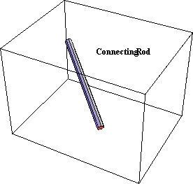
Out[39]= |  |
To show the complete quick-return mechanism, all of the graphics objects are put together and displayed subject to a Modeler3D solution rule. Here is the complete slider-crank mechanism at T = 0.10.
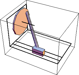
Out[40]= |  |
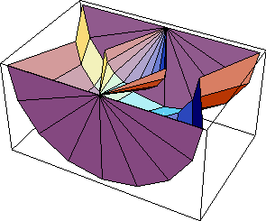
Here is the mechanism at T = 0.25, shown from a different perspective.
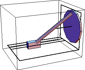
Out[41]= |  |
|