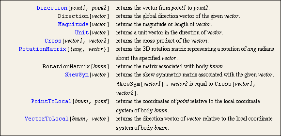
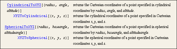
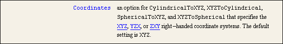
|
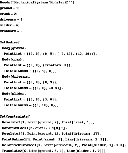
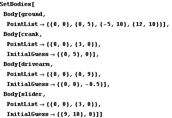
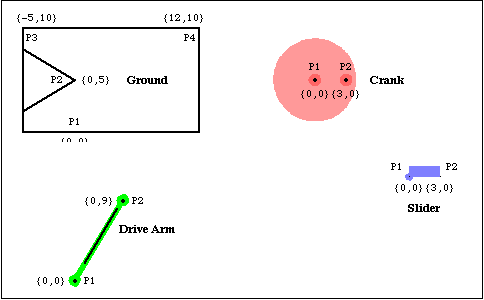
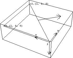
3. Output Functions OverviewThis chapter covers MechanicalSystems' numerical and graphical output functions. In general, Mech's output functions are used to convert the symbolic coordinates that define the location and orientation of each body into more specialized quantities, such as the distance between two points or the angle between two lines. Graphical output functions use the symbolic coordinates to locate graphics primitives to reflect the location of the bodies in the model. Throughout this chapter, Mech output functions are used as supplements to, not replacements for, built-in Mathematica functions. Most output from Mech is generated through a mixture of both. 3.1 2D Output FunctionsNumerical output from a Modeler2D model can be generated with output functions that are defined in the auxiliary package Graphics2D. This package is autoloaded after the Modeler2D main package has been loaded if any of the output functions are called. Each output function returns a symbolic expression that represents the quantity being sought, in terms of the model's dependent variables, X2, Y3, and so on. To achieve a numerical result, the dependent variables must be replaced with numbers, usually by applying a solution rule returned by SolveMech. More complicated and specific output functions can easily be defined by the user, making use of Mech's basic output functions and Mathematica's built-in vector algebra functions. 3.1.1 Example Mechanism To demonstrate the use of Modeler2D output functions, a 2D model is developed that can have various geometric quantities measured. The model is a planar quick-return mechanism consisting of three moving bodies: the crank, drive arm, and slider. A real quick-return mechanism would have a fourth body, the connecting rod between the drive arm and the slider, but this body is simply modeled with a relative-distance constraint.
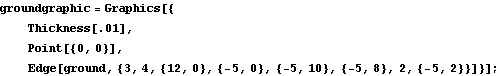
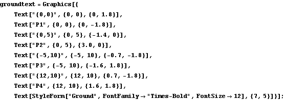
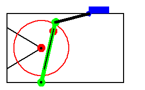
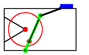
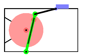
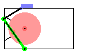
The motion of the quick-return mechanism is driven by the rotation of the crank that, in turn, forces the drive arm to rock about its lower pivot point on the ground, via a pin on the crank that slides in a straight slot on the drive arm. The top of the drive arm is attached to a connecting rod, which is attached to the slider, which slides on horizontal path on the ground. This loads the Modeler2D package. Here is a graphic of the 2D quick-return model.

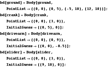
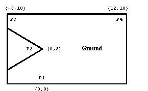
BodiesFour body objects are defined for the quick-return mechanism model. The ground (body 1) requires four point definitions.
P1 is the rotational axis of the drive arm.
P2 is the rotational axis of the crank.
P3 and P4 are two points that define the line upon which the slider slides.The crank (body 2) requires two local point definitions.
P1 is the crank's rotational axis.
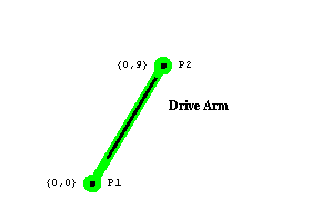
P2 is the location of the pin on the crank that engages with the drive arm.The drive arm (body 3) requires two local point definitions.
P1 is the point on the drive arm where the drive arm pivots with respect to the ground.
P2 is the point where the drive arm is attached to the pseudo-connecting rod.The slider (body 4) requires two local point definitions.
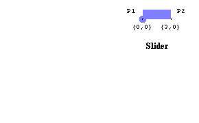
P1 and P2 are two points along the horizontal axis of the slider define its translation line.Here are the bodies in the quick-return model.
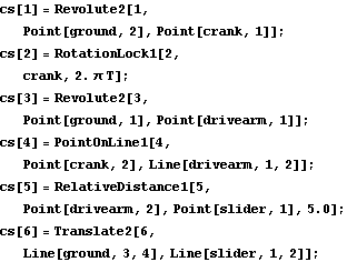
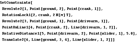
Names are defined for each of the body numbers in the mechanism. Body objects are defined for each body. This incorporates the body properties into the current model. ConstraintsFive constraints and one driving constraint are required to model the quick-return mechanism. A Revolute2 constraint forces the axis of the crank to be coincident with its pivot point on the ground. This constrains two degrees of freedom, X and Y displacement of the crank axis.A RotationLock1 constraint specifies the angular coordinate of the crank. This driving constraint is used to rotate the crank.A Revolute2 constraint forces the lower pivot point of the drive arm to be coincident with the global origin. The drive arm can pivot about this point on the ground.A PointOnLine1 constraint between the crank and the drive arm where the pin on the crank slides in a slot on the drive arm.A RelativeDistance1 constraint between the drive arm and the slider replaces the pseudo-connecting rod, which is 5.0 units long.A Translate2 constraint between the slider and the ground allows the slider to translate horizontally along a track on the ground.Here are five constraints for the quick-return model. This incorporates the constraints into the current model. RuntimeThis runs the model at T = 0.15
Out[18]= |  |
Here is the quick-return mechanism at T = 0.15.
3.1.2 Output FunctionsModeler2D numerical output functions return expressions that evaluate to numbers or vectors, such as the distance between two points, the angle between two lines, or the coordinates of a point. These functions take point, vector, and axis objects as arguments, identical in structure to the geometry objects used when building constraints. When local point numbers are used, the local coordinates are taken from the current body objects, as specified with SetBodies.
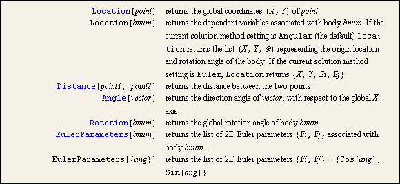
Each of the output functions are demonstrated in the context of the quick-return mechanism model defined in Section 3.1.1. Output functions. More complex output functions. The Location function is used to convert a Mech Point object into the global coordinates of the point. Here are the global coordinates of point 2 on the drive arm.
Out[19]= |  |
Location assumes a point object if only the arguments of Point are given.
Out[20]= |  |
This gets a numerical result from the output of Location.
Out[21]= |  |
Out[22]= |  |
The Distance function is used to find the absolute distance between any two points in space. The points can be on one body or on two different bodies. Here is the distance from the center of the crank to point 2 on the slider.
Out[23]= |  |
Here is the numerical result.
Out[24]= |  |
Here is the length of the line from the center of the crank to the drive pin.
Out[25]= |  |
Note that it was not necessary to apply a solution rule to the last example to get a numerical result because the dimension being measured is not a function of the coordinates of each body. Here is the minimum distance between the crank axis and the center line of the drive arm.
Out[26]= |  |
Now get a numerical result.
Out[27]= |  |
Note that the distance is zero when the crank has turned 1/4 turn, and the drive arm is pointed straight up, through the axis of the crank. Here is the direction angle of the center line of the connecting rod.
Out[28]= |  |
Now get a numerical result in degrees.
Out[29]= |  |
The Rotation function simply returns the angular coordinate of the specified body. Here is theta of the drive arm.
Out[30]= |  |
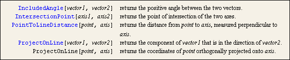
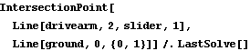
This returns the intersection of the connecting rod axis and a vertical line through the crank axis.
Out[31]= |  |
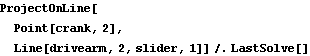
The ProjectOnLine function is used to find the projection of a point on one body onto a line located on another body (or bodies). This projects the crank's drive pin onto the connecting rod.
Out[32]= |  |
3.1.3 Vector Algebra FunctionsModeler2D vector algebra functions perform many common vector algebra operations such as cross and dot products of vectors. These functions can be used to build more complicated functions that are not provided by Modeler2D. The output functions take point, vector, and axis objects as arguments, identical in structure to the geometry objects used when building constraint objects. When local point numbers are used, the local coordinates are taken from the current body objects, as specified with SetBodies.
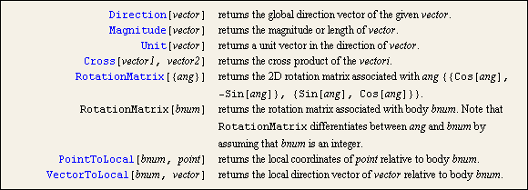
Each of the vector algebra functions are demonstrated in the context of the quick-return mechanism model defined at the beginning of this section. Vector algebra functions. The Direction function is used to convert Modeler2D vector objects into 2D vectors in global coordinates. Note that Mech's definition of Direction does not interfere with its use as a built-in Mathematica symbol. Here is the direction vector of the connecting rod.
Out[33]= |  |
Now get a numerical result.
Out[34]= |  |
Several Modeler2D output functions are textbook vector algebra functions that are capable of dealing with normal 2D vectors or Modeler2D line objects interchangeably. Magnitude can return the length of the line from one end of the connecting rod to the other.
Out[35]= |  |
Magnitude also works with simple vectors.
Out[36]= |  |
Unit also works with vectors or line objects.
Out[37]= |  |
The cross product of two vectors in 2D space is a scalar.
Out[38]= |  |
Now get a numerical result.
Out[39]= |  |
Here is a 2D rotation matrix that will rotate a vector on the slider into global coordinates.
Out[40]= |  |
The global coordinates of a point specified in a local reference frame are equal to the coordinates of the origin of the reference frame plus the local coordinates of the point, rotated into the global reference frame. Here is a calculation of the global coordinates of the local point {3, 8} on the slider.
Out[41]= |  |
The Location function performs effectively the same calculation, directly.
Out[42]= |  |
Now get a numerical result.
Out[43]= |  |
The PointToLocal function converts the global point back to local coordinates.
Out[44]= |  |
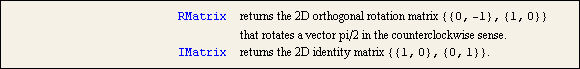
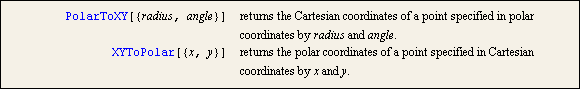
Two constant matrices that are commonly used in 2D vector algebra are also defined by Modeler2D. Constant utilities. Coordinate ConversionsPolarToXY and XYToPolar are two conversion functions that do not accept Modeler2D geometry objects as arguments. These functions only accept 2D vectors of the form {x, y}. Coordinate conversions. This converts a polar coordinate pair to Cartesian coordinates.
Out[45]= |  |
This converts it back.
Out[46]= |  |
This converts a 2D vector to polar coordinates.
Out[47]= |  |
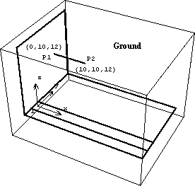
3.2 3D Output FunctionsNumerical output from a Modeler3D model can be generated with output functions that are defined in the auxiliary package Graphics3D. This package is autoloaded after the Modeler3D main package has been loaded if any of the output functions are called. Each output function returns a symbolic expression that represents the quantity being sought, in terms of the model's dependent variables X2, Z3, Ei4, and so on. To achieve a numerical result, the dependent variables must be replaced with numbers, typically by applying a solution rule returned by SolveMech. More complicated and specific output functions can easily be defined by the user, making use of Mech's basic output functions and Mathematica's built-in vector algebra functions. 3.2.1 Example Mechanism To demonstrate the use of Modeler3D output functions, a 3D model is developed that can be measured. The model is a spatial slider-crank mechanism consisting of two moving bodies, the crank and the slider. A real slider-crank mechanism would have a fourth body, the connecting rod between the crank and the slider.
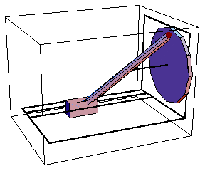
The motion of the slider-crank mechanism is driven by the rotation of the crank, which forces the slider to reciprocate in a straight track that is parallel to the axis of the crank. The crank is attached to the slider via a connecting rod that is modeled by a distance constraint. This loads the Modeler3D package. Here is a graphic of the complete 3D slider-crank model.
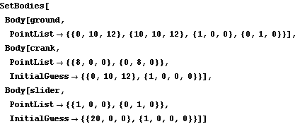
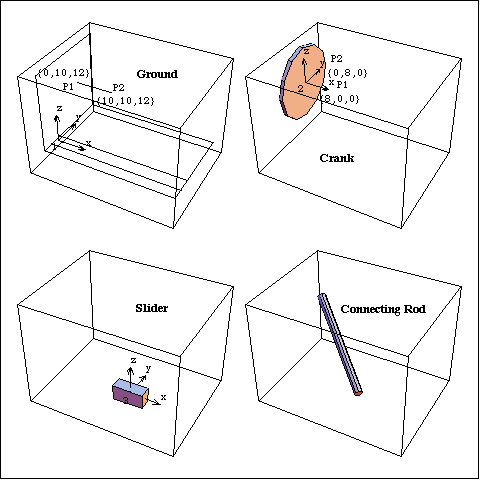
BodiesThree body objects are defined for the slider-crank mechanism model. Note that the zeroth point is used in this model to avoid repeatedly defining a point at coordinates {0, 0, 0}. The ground (body 1) has four points defined in its body object.
P1 and P2 are two points to define the rotational axis of the crank.
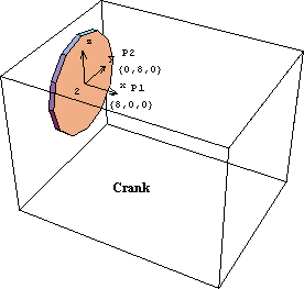
P3 and P4 are two points that are used in conjunction with the origin of the ground body to define the translation axis and reference direction of the slider. P4 is also used with the local origin to define a reference direction for the crank's rotation.The crank (body 2) has two points defined in its body object.
P1 is a point that is used with the crank's local origin to define its rotational axis.
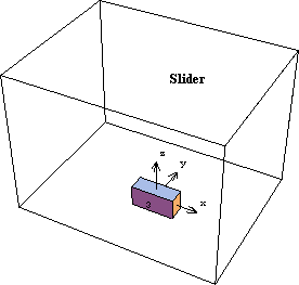
P2 is the attachment point of the connecting rod, and also a reference for the crank's rotation.The slider (body 3) has two points defined in its body object.
P0 is the attachment point of the connecting rod on the slider.
P1 is used with the slider's local origin to define its translation axis.
P2 is used with the slider's local origin to define a reference direction for the translational joint.Here are all the bodies in the slider-crank model.
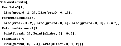
Here are names for each of the body numbers in the model. Here are body objects for each body. This incorporates the body properties into the current model. ConstraintsFour constraints are used to model the slider-crank mechanism. A Revolute5 constraint forces the axis of the crank to be coincident with its pivot axis on the ground. This leaves only one degree of freedom for the crank, rotation about its axis.A ProjectedAngle1 constraint specifies the angular relationship between a line on the ground body and a line on the crank. This driving constraint is used to rotate the crank.A RelativeDistance1 constraint between the crank and the slider replaces the pseudo-connecting rod, which is 30 units long.A Translate5 constraint between the slider and the ground leaves only one degree of freedom for the slider; horizontal translation along a track on the ground body. This constraint references two Modeler3D Axis objects that are constrained to be parallel and coincident, and the reference directions of the two axes are constrained to be coplanar.Here are the constraints for the slider-crank model. This incorporates the constraints into the current model. RuntimeNow run the model at T = 0.05.
Out[14]= |  |
Here is the slider-crank model at T = 0.05.
3.2.2 Output FunctionsModeler3D numerical output functions return expressions that evaluate to numbers or vectors, such as the distance between two points, the angle between two lines, or the coordinates of a point. These functions take Modeler3D point, vector, and axis objects as arguments, identical in structure to the geometry objects used when building constraints. When local point numbers are used, the local coordinates are taken from the current body objects, as specified with SetBodies.
Each of the output functions is demonstrated in the context of the quick-return mechanism model defined in Section 3.2.1. Output functions. More output functions. The Location function is used to convert a Mech point object into the global coordinates of the point. Here are the global coordinates of the attachment point of the connecting rod on the crank.
Out[15]= |  |
Location assumes a point object if only the arguments of Point are given.
Out[16]= |  |
Now get a numerical result.
Out[17]= |  |
Out[18]= |  |
The Distance function is used to find the absolute distance between any two points in space. The two points can be on one body or two different bodies. Here is the distance from a point on the axis of the crank to the origin of the slider.
Out[19]= |  |
Now get a numerical result.
Out[20]= |  |
Here is the length of the line from the center of the crank to the drive pin.
Out[21]= |  |
Note that it was not necessary to apply a solution rule to the last example to get a numerical result because the dimension that was measured was a constant. Here is the minimum distance between the crank axis and the center line of the connecting rod.
Out[22]= |  |
Here is the angle between the connecting rod and the crank axis.
Out[23]= |  |
Now convert the previous result to degrees.
Out[24]= |  |
The measure of an angle in 3D space requires a reference frame for measurement. ProjectedAngle allows the plane of projection of the angle to be specified. Here is the angle of a line on the crank, relative to a line on the ground, as viewed looking down the crank axis.
Out[25]= |  |
Now get a numerical result at T = 0.35.
Out[26]= |  |
This angle should be equal to 35/100 of a turn, since that is what we have specified with SolveMech.
Out[27]= |  |
This finds the intersection of the connecting rod axis and a horizontal plane through the crank axis.
Out[28]= |  |
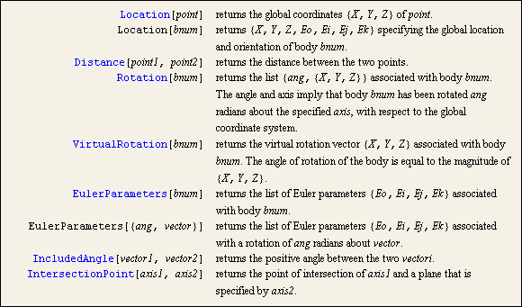
The angular orientation of a body in 3D space can be uniquely specified by a single rotation about a fixed axis. Rotation returns the angle and axis associated with the current spatial orientation of a body. See Section 4.2 for more examples on the angular orientation of 3D bodies. This finds the angle and axis of rotation of the crank.
Out[29]= | 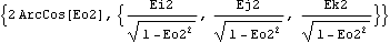 |
Now get a numerical result.
Out[30]= |  |
3.2.3 Vector Algebra FunctionsModeler3D vector algebra functions perform many common vector algebra operations, such as cross and dot products of vectors. These functions can be used to build more complicated functions that are not provided by Modeler3D. These functions take point, vector, and axis objects as arguments, just like the output functions described in Section 3.2.2. When local point numbers are used, the local coordinates are taken from the current body objects, as specified with SetBodies.
Each of the vector algebra functions is demonstrated in the context of the slider-crank mechanism model defined at the beginning of this section. Vector algebra functions. The Direction function is used to convert Modeler3D vector objects into 3D vectors in global coordinates. Here is the direction vector of the connecting rod.
Out[31]= | 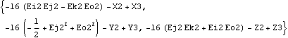 |
Now get a numerical result.
Out[32]= |  |
Several Modeler3D output functions are textbook vector algebra functions that are capable of dealing with normal 3D vectors or Modeler3D vector/axis objects interchangeably. Magnitude can return the length of the line from one end of the connecting rod to the other.
Out[33]= |  |
Here is the length of a simple 3D vector.
Out[34]= |  |
Unit also works with vectors or vector objects.
Out[35]= |  |
The cross product of two vectors is found with the Cross function. Here is the cross product of a Modeler3D Line object and a vector.
Out[36]= |  |
Now get a numerical result.
Out[37]= |  |
Here is the 3D rotation matrix associated with the crank.
Out[38]= |  |
Here is the skew symmetric matrix operator.
Out[39]= |  |
The global coordinates of a point specified in a local reference frame are equal to the coordinates of the origin of the reference frame plus the local coordinates of the point, rotated into the global reference frame. Here is a calculation of the global coordinates of the local point {3, 8} on the slider.
Out[40]= |  |
The Location function performs effectively the same calculation.
Out[41]= |  |
The PointToLocal function converts the global point back to local coordinates.
Out[42]= |  |
A constant utility. Coordinate ConversionsThe following four conversion functions will not accept Modeler3D geometry objects as arguments. These functions only accept 3D vectors of the form {x, y, z}. Coordinate conversions. Coordinate conversion options. This converts a cylindrical coordinate triplet to Cartesian coordinates.
Out[43]= |  |
This converts it back.
Out[44]= |  |
This converts a 3D vector to polar coordinates.
Out[45]= |  |
3.3 Plots and GraphsThis section discusses various methods for generating plots of Mech output. Because Mech uses a numerical technique to solve the kinematic equations that make up a mechanism model, it is generally not possible to generate analytic expressions that represent geometric quantities in a model that are to be plotted. The best that can be done is to generate a series of discreet solutions to the mechanism model, and then use the solutions to create lists of numbers that are plotted using Mathematica's built-in data plotting routines such as ListPlot, or interpolated using Mathematica's InterpolatingFunction. 3.3.1 Example MechanismThe quick-return mechanism model that was developed in Section 3.1 is used here to demonstrate all of the plotting techniques in this chapter. The model is redefined as follows in abbreviated form.
Note that a parameter crankarm has been added to the model to allow the position of the drive pin on the crank to be easily changed. Here is the entire quick-return model. A graphic of the quick-return mechanism.
3.3.2 Data PlotsTo generate a data plot, we must first generate some data. SolveMech is used to return 20 solution points as the crank is rotated through a full turn, with the crank arm length set to three units. This generates a list of 20 solutions.
Out[10]= |  |
Since the primary function of the quick return mechanism is to reciprocate the slider, the X position of the slider is plotted as a function of time. Each solution rule returned by SolveMech contains a rule specifying the value of time T so a list of {x, y} pairs for ListPlot can easily be obtained with one replacement operation. Here is a plot of slider position versus time.
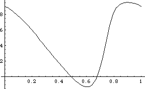
Out[11]= |  |
More complicated functions can also be plotted in this manner. Here is a plot of connecting rod angle versus time.
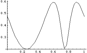
Out[12]= |  |
To create a series of plots while varying the value of crank arm, the Table function is used in conjunction with SolveMech to generate a nested list of solutions. Note that at each invocation of SolveMech the value of time T is taken from 0 to 1, which takes the angular coordinate of the crank  2 from 0 to 2 pi. This requires the value of 2 to jump from 2 pi back to 0 in one step at each new invocation of SolveMech, which is a rather large single step for the numerical solution method. To avoid possible numerical difficulties, the initial guesses are reset with SetGuess at each invocation of SolveMech. 2 from 0 to 2 pi. This requires the value of 2 to jump from 2 pi back to 0 in one step at each new invocation of SolveMech, which is a rather large single step for the numerical solution method. To avoid possible numerical difficulties, the initial guesses are reset with SetGuess at each invocation of SolveMech. This generates a nested list of solutions. To generate a series of plots a rather obtuse invocation of ListPlot is used. This shows a plot of slider position at varying values of crankarm.
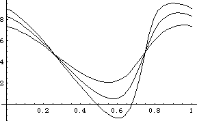
Out[14]= |  |
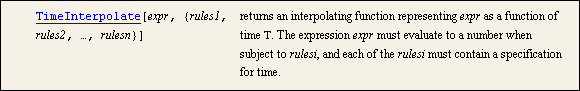
3.3.3 InterpolationMathematica InterpolatingFunction objects can be used to improve the appearance of a ListPlot by smoothing out the data. Mech provides a function that facilitates the creation of InterpolatingFunction objects, by assuming a dependence on time. Mech interpolation utility. Using the quick-return mechanism model that was defined in Section 3.3.1, the plot of the connecting rod angle is reproduced using TimeInterpolate to create an InterpolatingFunction. This generates a list of solutions. This generates an InterpolatingFunction object.
Out[18]= |  |
Here is a plot of the connecting rod angle versus time.

Out[19]= |  |
3.4 2D Mechanism ImagesThis section demonstrates special Modeler2D graphics functions that are used to generate the mechanism images throughout this document. Modeler2D graphics functions return graphics primitives that are given as arguments to the Mathematica Graphics function and displayed with the Show command, just like the built-in Mathematica graphics primitives.
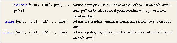
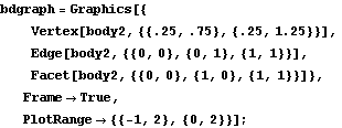
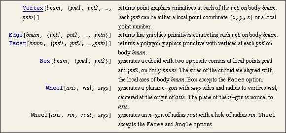
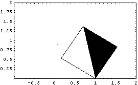
The primary utility of the Modeler2D graphics functions is that they take their arguments in the form of local coordinates and automatically convert them to global. Thus, it is possible to create the image of a mechanism part using the same techniques as would be used with built-in Mathematica graphics primitives, and then have the part be positioned properly with respect to the other parts of the mechanism automatically, as specified by a Modeler2D solution rule returned by SolveMech. 3.4.1 Graphics FunctionsThe Modeler2D graphics functions closely parallel the built-in Mathematica graphics primitives. Each graphics function generates Mathematica graphics primitives that represent points, lines, or polygons. Basic Mech graphics function. More 2D graphics functions. Options for graphics functions. The Modeler2D Vertex, Edge, and Facet functions are analogous to the built-in Mathematica Point, Line, and Polygon functions. To demonstrate these functions, graphics objects are generated that are located on body 2, which is named body2. This loads the Modeler2D package. Here is a box with a diagonal and a couple of points. The coordinates of the graphic just created bdgraph are functions of the Modeler2D variables that locate body2: X2, Y2, and 2. Therefore, these variables must be replaced with numeric values before the graphic can be displayed with Show. This shows bdgraph rotated 0.5 radians counterclockwise.
Out[5]= |  |
This shows bdgraph rotated 1 radian and translated 1 unit to the right.
Out[6]= |  |
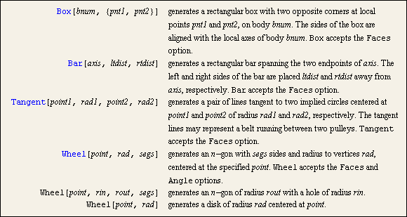
The Box function is analogous to the built-in Rectangle function, with the exception that the sides of the Box graphic are aligned with the local coordinate system in which the graphic is located, instead of being aligned with the global coordinate system.
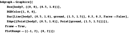
The Bar function also generates a rectangular box, but instead of specifying two points on two opposite corners, two points on two opposing sides of the rectangle are specified. The Faces option is used with the Bar function to show only an outline of the bar. Unlike the Box function, Bar accepts an axis object as its first argument, to allow the two endpoints of the bar to lie on two different bodies. Here is a Box graphic on body2 and a Bar graphic spanning from body2 to the ground, with an Edge graphic down the middle. Here is the result.
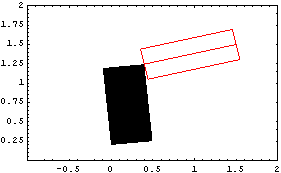
Out[8]= |  |
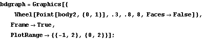
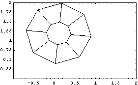
The Wheel function is used here to generate an octagon with a hole in it. Note that the n-gon returned by Wheel is placed on the body that is referenced in the Point argument, and is located with that body as such. This generates an octagon on body2. Here is the result.
Out[10]= |  |
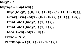
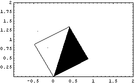
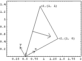
3.4.2 Annotation FunctionsThree graphics functions are provided by Modeler2D specifically for annotation. Graphics functions for annotation. PointLabel and LocalAxes can be used to conveniently label points and bodies. The following input generates a triangle placed on body 2, with two of the points labeled with their body numbers and local coordinates. This generates a labeled triangle on body2. Here is the result.
Out[13]= |  |
A function for plotting the locus of a moving point. The nested list of rules required by LocusPlot is of the form returned by SolveMech when given a range of times at which to seek solutions. 3.4.3 Example Mechanism GraphicsThe quick-return mechanism model that was developed in Section 3.1 is used to demonstrate the Modeler2D graphics functions. The model is redefined as follows in abbreviated form. The complete quick-return model. To demonstrate the use of the graphics functions, the image of the quick-return mechanism that was displayed in the preceding sections is built. These images are generated with a mix of Modeler2D graphics functions and built-in Mathematica graphics primitives. GroundThe ground body of the quick-return mechanism is generated using Modeler2D graphics functions even though it does not move. This is done to take advantage of the easy referencing of local point coordinates that were defined with SetBodies. Note that the Edge function in the following graphic references points either by their {x, y} coordinates or by their local point numbers interchangeably. Here is the ground body graphic. The text that is shown with the ground body is generated entirely with the built-in Mathematica Text function. Here is the ground body graphic annotation. Here is the result.
Out[22]= |  |
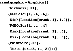
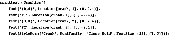
CrankThe crank graphic uses only built-in Mathematica graphics functions, with the exception of the Vertex function to plot two local points on the crank, the coordinates of which are defined in a body object. Note the use of the Location function inside of the Disk primitives. This places the disks at the correct global coordinates when the crank moves. Here is the crank body graphic. The text that is displayed with the crank graphic also uses the Location function to specify the global coordinates of the text so that the text moves with the crank. Here is the crank graphic annotation. Because the coordinates of some of the elements in crankgraphic and cranktext are now functions of Modeler2D dependent variables X2, Y2, and 2, a Modeler2D solution rule must be applied before they can be displayed. Note the use of SolveMech in the following input. Here is the result.

Out[25]= |  |
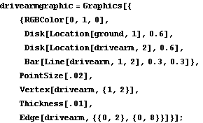
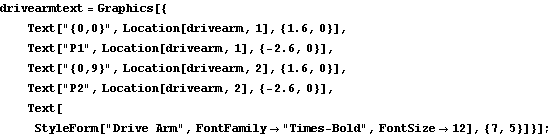
Drive ArmThe drive arm graphic uses mostly built-in Mathematica graphics functions. Note how the Bar and Vertex function are called using local points 1 and 2, while the Edge function is called with explicit local point coordinates {0, 2} and {0, 8}. Most Mech functions attempt to interpret integers as local point numbers and resolve them into coordinates. Here is the drive arm graphic. The text that was displayed with the drive arm graphic also used the Location function to specify the global coordinates of the text so that the text moves with the drive arm. Here is the drive arm graphic annotation. Like the crank graphic, the coordinates in the drive arm graphic are functions of Modeler2D dependent variables. Thus, a solution rule must be applied to display the graphic. Here is the result.
Out[28]= |  |
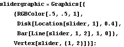
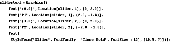
SliderThe slider graphic uses just one built-in Mathematica graphics primitive and one Modeler2D graphics function. Here is the slider graphic. Here is the slider annotation. Here is the result.
Out[31]= |  |
Connecting RodThe connecting rod graphic is nothing more than a line connecting two points on two different bodies. Here is the connecting rod graphic. To show the complete quick-return mechanism, all of the graphics objects are combined and displayed subject to a single Modeler2D solution rule. Here is the complete mechanism at T = 0.15.
Out[33]= |  |
Here is the mechanism at T = 0.55.
Out[34]= |  |
3.5 3D Mechanism ImagesThis section demonstrates the special Modeler3D graphics functions that are used to generate the mechanism images throughout this document. Modeler3D graphics functions return graphics primitives that are given as arguments to the Mathematica Graphics function and displayed with the Show command, just like the built-in Mathematica graphics primitives.
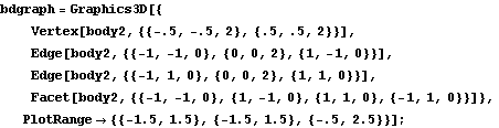
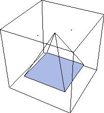
The primary utility of the Modeler3D graphics functions is that they take their arguments in the form of local coordinates and automatically convert them to global. Thus, it is possible to create the image of a mechanism part using the same techniques as would be used with built-in Mathematica graphics primitives, and then have the part be positioned properly with respect to the other parts of the mechanism automatically, as specified by a Modeler3D solution rule. 3.5.1 Graphics FunctionsThe elementary Modeler3D graphics functions closely parallel the built-in Mathematica graphics primitives. Each graphics function generates Mathematica graphics primitives that represent points, lines, or polygons. The Modeler3D compound graphics functions generate more complex shapes, such as spheres and cylinders. Basic 3D graphics functions. More 3D graphics functions. Options for graphics functions. The Modeler3D Vertex, Edge, and Facet functions are analogous to the built-in Mathematica Point, Line, and Polygon graphics primitives. To demonstrate these functions, graphics objects are generated on body 2, which is named body2. This loads the Modeler3D package. Here is a pyramid with a filled floor. The coordinates of the graphic just created bdgraph are functions of the Modeler3D variables that locate body2: X2, Y2, Z2, Eo2, Ei2, Ej2, and Ek2. Therefore, these variables must be replaced with numeric values before trying to Show the graphic. Here is bdgraph located coincidentally with the local origin.
Out[5]= |  |
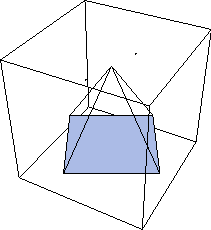
To show the pyramid in another orientation, a set of four Euler parameters are fabricated that represent the desired angular orientation. Normally, Modeler3D graphics functions are used in conjunction with a Modeler3D solution rule that contains the values of the Euler parameters needed, but in this case they are generated explicitly.
The pyramid is now rotated 0.5 radians about the global Z axis. The EulerParameters function returns the Euler parameters required for this rotation. These Euler parameters represent a rotation of 0.5 radians about the {0, 0, 1} axis.
Out[6]= |  |
Now the parameters are turned into rules for Eo2, Ei2, Ej2, and Ek2.
Out[7]= |  |
Here is bdgraph rotated 0.5 radians about the Z axis.
Out[8]= |  |
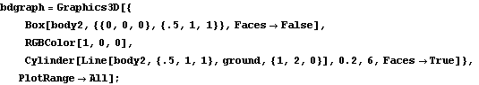
The Box function is analogous to the built-in Cuboid function, with the exception that the sides of the Box graphic are aligned with the local coordinate system on which the graphic is located, instead of being aligned with the global coordinate system.
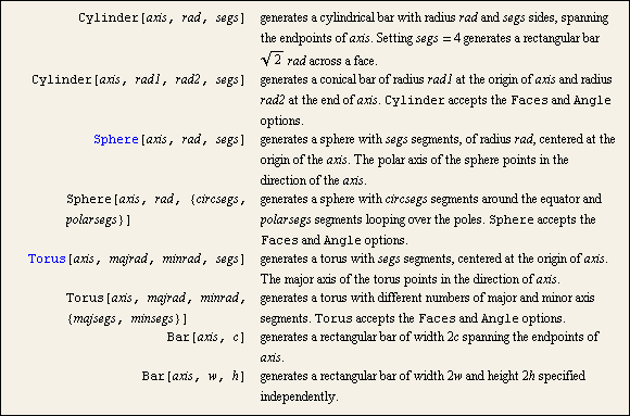
The Cylinder function generates a faceted cylinder or cone, with endpoints located at the two ends of a Modeler3D line object. The Faces option is used with Cylinder to show only an outline of the cylinder. Here is a Box graphic on body2 and a Cylinder graphic spanning from body2 to the ground. Here is the result.
Out[10]= |  |
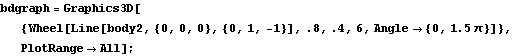
The Wheel function is used here to generate a part of an octagon with a hole in it. Note that the n-gon returned by Wheel is placed on the body that is referenced in the Point argument, and is located with that body as such. This generates a piece of an octagon on body2. Here is the result.
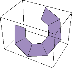
Out[12]= |  |
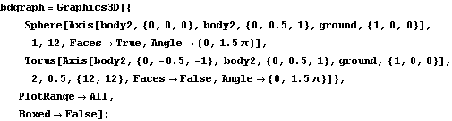
The Sphere and Torus functions are used here to generate a sphere and a torus. This generates a piece of a sphere and a torus on body2. Here is the result.
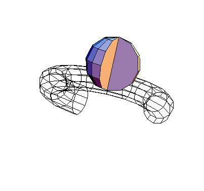
Out[14]= |  |
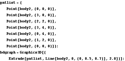
Functions to generate pseudo-solid objects. Extrude is used to generate a sequence of faces that are defined by sweeping a sequence of connected lines through 3D space. The following example takes six points on body2 that define an hourglass form and extrudes them at an oblique angle into a set of six facets forming a canted hourglass. Here are the points for an hourglass graphic. The graphic is shown shifted 2 units in the Y direction off of the global origin.
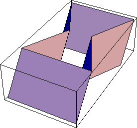
Out[17]= |  |
The same list of points can be revolved about an axis specified on body2. Here is a revolution of the hourglass graphic. Here is the result.
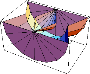
Out[19]= |  |
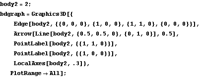
3.5.2 Annotation FunctionsThree graphics functions are provided by Modeler3D specifically for annotation. Graphics functions for annotation. PointLabel and LocalAxes can be used to conveniently label points and bodies. The following input generates a triangle placed on body 2, with two of the points labeled with their body numbers and local coordinates. This generates the triangle graphic. Here is the result.
Out[22]= |  |
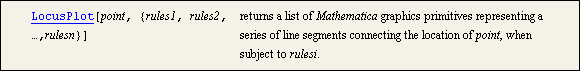
A function for plotting the locus of a moving point. The nested list of rules required by LocusPlot is of the form returned by SolveMech. 3.5.3 Example Mechanism GraphicsThe spatial slider-crank mechanism model that was developed in Section 3.2 is used to demonstrate the use of Modeler3D graphics functions to create an image of a mechanism model. Creating a complex mechanism image often requires more lines of Mathematica code than were used in the kinematic model of the mechanism. This is because of the terse nature of the data required to kinematically describe a mechanism. A kinematic model uses only a small number of points in space to define rotational and translational axes that tie the bodies together, while the mechanism image requires much more information about the shape of the bodies in the model.
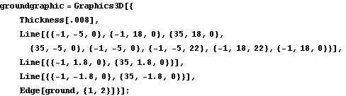
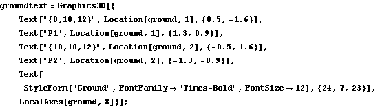
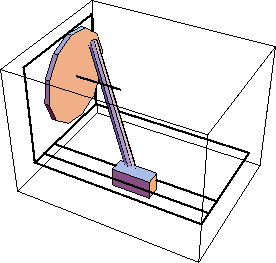
The spatial slider-crank model is redefined as follows in abbreviated form. See Section 3.2 for a full description of this mechanism model. Here is the complete definition of the slider-crank model. To demonstrate the use of the graphics functions the image of the slider-crank mechanism that is displayed in the preceding sections is built. These images are generated with a mix of Modeler3D graphics functions and built-in Mathematica graphics primitives. GroundThe ground body of the slider-crank mechanism was generated using mostly built-in Mathematica graphics primitives. The Modeler3D Edge function was used to generate a line on the crank axis referencing local points by their point numbers. Here is the ground body graphic. The text that was displayed with the ground body was generated entirely with the built-in Mathematica Text function, except for the axes at the global coordinate origin, generated with the Modeler3D LocalAxes function, and the use of the Location function to reference the global coordinates of local point numbers on the ground body. Here is the ground body annotation. Here is the result.
Out[30]= |  |
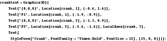
CrankThe crank graphic uses the Modeler3D Cylinder function to generate a very short cylinder. The cylinder is only one unit long because the line that defines its axis is one unit long, while the radius of the cylinder is ten units as specified. Here is the crank body graphic. The text that was displayed with the crank graphic also used the Location function to specify the global coordinates of the text so that the text moves with the crank. Here is the crank annotation. Because the coordinates of some of the elements in crankgraphic and cranktext are now functions of Modeler3D dependent variables, X2, Y2, and so on, a Modeler3D solution rule must be applied before they can be displayed. Note the use of SolveMech in the following input. The rules that are returned by SolveMech determine where the crank is located in 3D space. Here is the result.
Out[33]= |  |
SliderThe slider graphic uses the Modeler3D Box function to generate the rectangular box form of the slider. Here is the slider graphic. Here is the slider annotation. Like the crank graphic, the coordinates in the slider graphic are functions of Modeler3D dependent variables. Thus, a solution rule must be applied to display the graphic. Show it.
Out[36]= |  |
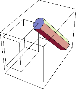
Connecting RodThe connecting rod graphic uses the Modeler3D Cylinder function again to generate a long, thin cylinder spanning from the crank to the slider. Here is the connecting rod graphic. Here is the connecting rod annotation. Here is the result.
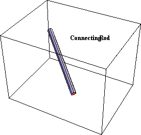
Out[39]= |  |
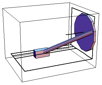
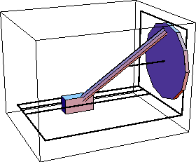
To show the complete quick-return mechanism, all of the graphics objects are put together and displayed subject to a Modeler3D solution rule. Here is the complete slider-crank mechanism at T = 0.10.
Out[40]= |  |
Here is the mechanism at T = 0.25, shown from a different perspective.
Out[41]= |  |
|