10.4.3 Free Response

To find the free acceleration of the pendulum, a FreeSystem object is built that contains a new set of equations of motion with constraints 5, 6, and 7 dropped from the model. Note that no initial conditions are yet available for the velocity of the bodies in the model. SetFree sets all of the initial velocities to zero if none are specified with the InitialCondition option.

This drops the constraints that lock the position of the pendulum. SetFree needs initial conditions for the velocity of each body. Since none are available zero is assumed.

In[6]:=

This integrates the FreeSystem object from T = 0 to T = 4.5, which is approximately a full period of the pendulum. The MakeRules option includes the velocity solution in the result.

In[7]:=

Here is a plot of the X coordinates of the slider and the pendulum.

In[8]:=

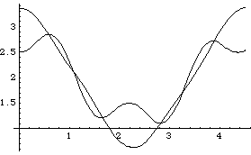
Out[8]=

Since the pendulum model is a conservative system, the sum of the kinetic and potential energy in the system should remain constant. This fact can be used to measure the accuracy of the numerical integrator.

A special output function.

The kinetic energy of each body is given by the BodyEnergy function, and the potential energy is simply the gravitational potential energy mass G altitude. The following plot shows that the numerical error in the integration has allowed the total energy of the model to increase by about 0.04% over 4.5 seconds.

Here is the total energy in the pendulum model.

In[9]:=

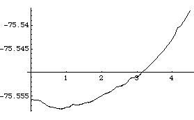
Out[9]=

Tightening the error budget by a factor of 100 by specifying the MaxError -> 0.000001 option for SolveFree will reduce the total energy rise to only 0.0007%, over the same time period, with an associated doubling of run time. Using the ConstraintCorrection -> True option, with the default error budget, will reduce the total energy rise to 0.002% with a slightly smaller increase in run time. In this case, either constraint correction or reducing step size (which is the result of decreasing the error budget) gives similar returns on computer time investment.
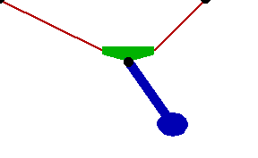
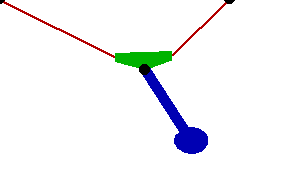
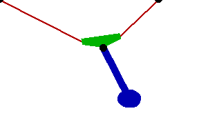
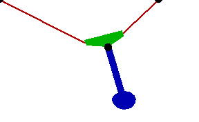
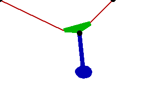
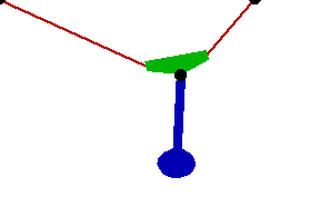
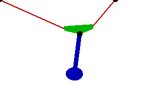
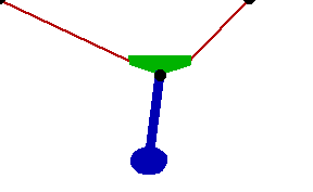
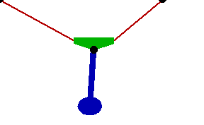
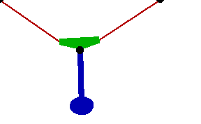
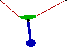
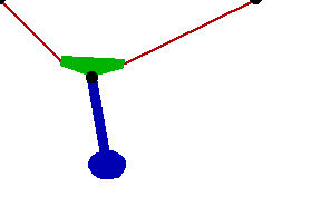
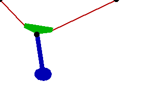
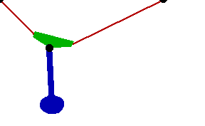
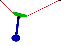
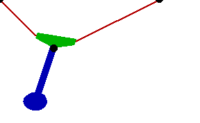
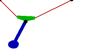
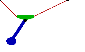
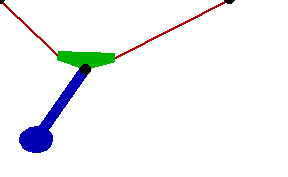
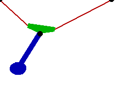
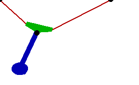
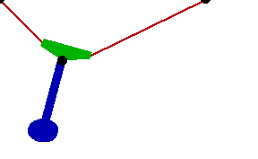
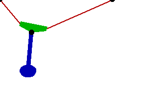
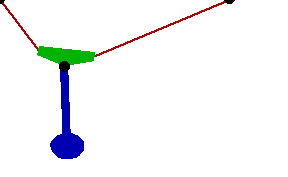
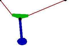
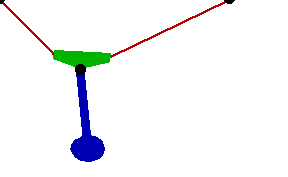
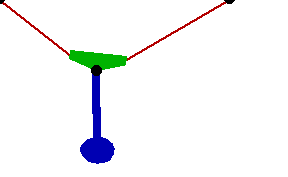
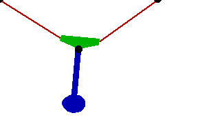
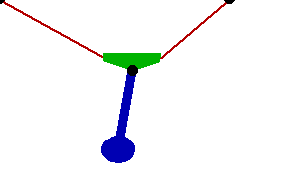
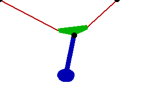
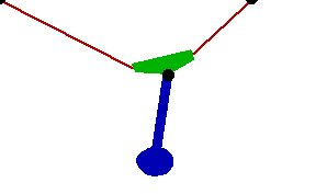
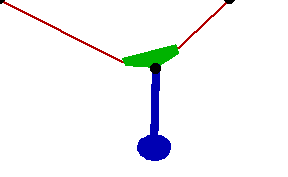
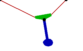
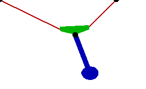
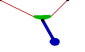
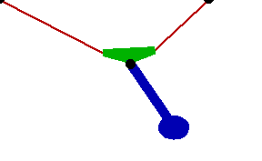
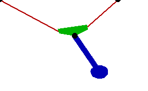
Changing the FitDegree setting can also affect the integration error. Setting FitDegree to Quadratic for this example will increase the net energy rise to 0.08%, while setting FitDegree to Quartic will reverse the sign of the error, changing the net energy rise to - 0.04%. Specifying a higher FitDegree setting often produces unexpected results because the automatic time step size adjustment works to counteract the higher degree setting. The integrator measures a smaller error in each step so it chooses a larger step size, resulting in the same net error.

Here is the pendulum-on-a-rope model at T = 1, 2, and 3 seconds.

Here is an animation of the pendulum-on-a-rope model.