10.3.5 Gyroscopic MomentsGyroscopic forces and moments modeled as per the example in Section 10.3.4 work well for single point analyses. However, if the time-domain free response is desired, such a modeling technique has a serious computational problem. While the rotor is spinning rapidly, the Euler parameters that represent the angular orientation of the rotor are changing sinusoidally and very rapidly. To numerically integrate such a system, the integrator must faithfully track very many periods of the sinusoidal Euler parameters to cover only a few periods of the motion of the more interesting parts of the gyroscope. If the period of the rotor's local rotation is much, much shorter than the period of interest, the integration becomes computationally infeasible.
The way around this problem is to introduce a special forcing function that mimics the gyroscopic torque of a spinning axially symmetric body and apply it to the rotor. This allows the rotor to be rotationally static.
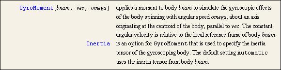
A function to simulate gyroscopic moments. GyroMoment has two important caveats attached to its use: the gyroscopic motion that it models is that of a body rotating about a principal axis of inertia and the two principle moments not associated with the axis of rotation must be equal. For most practical purposes, this means that the body is axially symmetric, and it is rotating about its axis of symmetry.
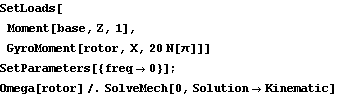
To demonstrate the use of GyroMoment, the gyroscope model that was presented in Section 10.3.3 is modified to remove the large angular velocity of the rotor and replace it with a GyroMoment load. Here the gyroscopic moment simulation is added to the applied loads, the angular speed of the rotor body is reduced to zero, and the model is run at T = 0 so initial conditions are available to SetFree.
Out[40]= |  |
First, the constraint that locks the base to the ground is dropped and SolveFree is run with the Z direction angular velocity set to 1. The resulting angular velocities and accelerations are missing the large components that were due to the rotation of the rotor.
Out[43]= |  |
But the reaction at the base still reflects the gyroscopic torques.
Out[44]= |  |
This builds and solves the FreeSystem object with constraints 2 and 4 dropped. Without the rotation of the rotor, the angular accelerations of the rotor and gimbal are equal.
Out[47]= |  |
There is still no gyroscopic torque applied to the base when the gimbal is free to rotate.
Out[48]= |  |
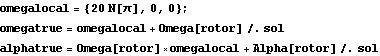
The constraint reaction forces that result from using this method are identical to the reaction forces that result from the normal procedure, without the use of GyroMoment. The true values of alpha and omega for the simulated rotor are reproduced by the following calculation. omegalocal is the local angular velocity vector that was passed to GyroMoment. Note that omegatrue and alphatrue match the angular velocity and acceleration components of the rotor in the previous analysis.
Out[50]= |  |
Out[51]= |  |
The equations of motion that are produced by this method are essentially equivalent to the equations of motion without the spinning rotor simulation, with one important difference, these equations of motion can be easily integrated to obtain the time-domain motion of the entire gyroscope assembly without an overwhelming computational burden.
|