10. Underconstrained Systems

Overview

This chapter covers MechanicalSystems' SetFree and SolveFree functions, which are used to synthesize the dynamic motion of underconstrained mechanical systems. SolveFree uses an adaptive multistep integration algorithm to integrate the equations of motion built by SetFree, and returns the dynamic motion profile of the model in the form of standard Mathematica interpolating functions. SetFree and SolveFree are also used to find the equilibrium configuration of underconstrained models that are subject to conservative static loading, or the equilibrium velocity of underconstrained models subject to velocity-dependent loading.
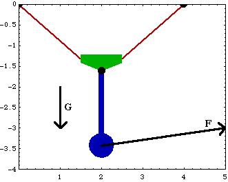
The SetPath and SolvePath functions are used to find the motion trajectories of models with one or more nonholonomic constraints. All Mech models must first be defined as fully constrained systems with SetConstraints before they can be modified with SetFree or SetPath.

10.1 Equilibrium Configuration

This section describes the use of the SetFree and SolveFree functions to find the equilibrium configuration of an underconstrained mechanism subject to static forces. A planar model of a pendulum sliding on a massless rope is used to demonstrate the use of SetFree and SolveFree.

10.1.1 Example Mechanism

The pendulum-on-a-rope model in the following example consists of two planar bodies, a slider that moves without friction along an infinitely flexible, inextensible, massless rope, and a pendulum that hangs below the slider and is attached to the ground by a spring. Before an equilibrium analysis can be done, the model must have a full set of kinematic constraints so that it can be assembled and each body can be moved to a reasonable position to use as an initial guess for the equilibrium analysis. Some of these kinematic constraints are then dropped to make the model underconstrained.

This loads the Modeler2D package and turns off the general spelling warnings.

In[1]:=

Bodies

Three body objects are defined for the pendulum model. Note that the zeroth point, which is defined to be {0,0} by default, is used in each body.

Names are defined for each of the body numbers.

In[4]:=

Here are the three body objects, including inertia properties.

In[7]:=

Constraints

Seven constraints are used to model the pendulum-on-a-rope model.

Here are the seven constraint objects for the pendulum-on-a-rope model.

In[8]:=

Runtime

Because there is no occurrence of time T in the model, the model can be run with the SolveMech command with no time argument. Since there are no other symbolic parameters, the model can only achieve one configuration, the one specified by the constraints.

Now the model is run with SolveMech.

In[9]:=

Out[9]=

Here is the pendulum-on-a-rope model in its initial configuration.

Forces

A model must have some nonzero loads applied to it in order to have a unique equilibrium position. The pendulum-on-a-rope model has three forces applied to it: a spring force applied to the pendulum, and gravity applied to the pendulum and the slider.

Here are the loads applied to the pendulum and slider.

In[10]:=

Here is the reaction to constraint 7 that prevents the pendulum from rotating. The constraint applies a clockwise moment to the pendulum to constrain it against the force of the spring.

In[11]:=

Out[11]=

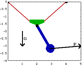
10.1.2 Finding Equilibrium

To find the equilibrium configuration of a mechanism, a FreeSystem object is built that contains a new set of equations of motion with one or more constraints removed from the model.

Finding equilibrium configuration.

The pendulum-on-a-rope model has three constraints that are present only to complete the kinematic model, constraints 5, 6, and 7. Each of these constraints is dropped, one at a time, and the equilibrium position is found with each new degree of freedom. The first constraint to be dropped is constraint 7, which locks the rotation of the pendulum relative to the slider. This allows the pendulum to rotate, but the slider stays locked at the center of the rope.

This drops constraint 7.

In[12]:=

Out[12]=

This solves the FreeSystem object.

In[13]:=

Out[13]=

Here is the pendulum model with constraint 7 dropped.

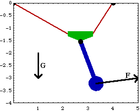
Next, constraint 5 is dropped, allowing the slider to move along the rope. Finally, constraint 6 is dropped, allowing the slider to rotate. The InitialGuess option is used to pass SetFree the solution to the last FreeSystem, which is named sol. This solution is a better initial guess than the defaults pulled from LastSolve[].

An option for SetFree.

Here is another FreeSystem object with constraints 5 and 7 dropped.

In[14]:=

This solves the FreeSystem object. Note that X2 has increased because the slider has moved to the right.

In[15]:=

Out[15]=

Here is the equilibrium position with constraints 5 and 7 dropped.

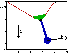
Here a FreeSystem object with constraints 5, 6, and 7 dropped is built and solved.

In[16]:=

Out[17]=

Here is the complete equilibrium position of the pendulum-on-a-rope model.

This returns MechanicalSystems to its initial state.

In[18]:=

Undocumented Graphics Generation

10.2 Equilibrium Velocity

This section covers the use of the SetFree and SolveFree functions to find the equilibrium velocity of a mechanism that has velocity-dependent loading. A mechanism must have some loading that is a direct function of velocity for it to have a defined equilibrium velocity. Note that the centrifugal forces in a model, although they are explicitly functions of velocity, are inertial forces and do not appear in a velocity equilibrium analysis.

10.2.1 Example Mechanism

This simple planar slider-crank model is presented with little explanation because all of the techniques used in the model have been explored in previous chapters.
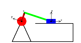
The one feature of interest in this model is the velocity-dependent applied loading. Two loads are applied, a driving moment on the crank and a viscous friction on the slider. Note that the driving moment applied to the crank is a function of velocity such that the moment drops to zero as velocity increases. This is done so that the velocity will not approach infinity when the piston is not moving at top-dead-center and bottom-dead-center.

This loads the Modeler2D package and defines names for each of the body numbers.

In[1]:=

Here are the constraints for the slider-crank model.

In[5]:=

Here are the velocity-dependent applied loads. Note that the force on the slider always opposes its direction of motion.

In[7]:=

Here is the moment that is applied to the crank by the rotational constraint at T = 0.2.

In[8]:=

Out[8]=

Here is the slider-crank model at T = 0.2.

10.2.2 Finding Equilibrium Velocity

To find the equilibrium velocity of a mechanism, a FreeSystem object is built that contains a new set of equations of motion with one or more constraints removed from the model.

Velocity equilibrium.

The driving constraint is dropped from the slider-crank model to give the model one degree of freedom.

This drops the constraint that controls rotation of the crank.

In[9]:=

This solves the FreeSystem object. Note that the angular velocity of the crank 2d is less than the driven angular velocity of 2 pi.

In[10]:=

Out[10]=

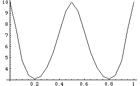
To find the equilibrium velocity at a sequence of positions through a full cycle of the mechanism, the InitialCondition option is used to pass SolveFree a new set of initial conditions at each position where the equilibrium velocity is to be found. Thus, it is not necessary to create a new FreeSystem object for each solution point.

An option for SetFree and SolveFree.

This generates a list of 20 rules to be used as initial conditions for the equilibrium velocity solution.

In[11]:=

This solves the FreeSystem object at each initial condition in postab.

In[13]:=

Here is a plot of the equilibrium velocity of the crank through a full cycle of the mechanism.

In[14]:=

Out[14]=

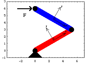
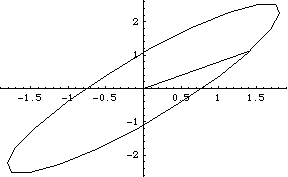
Undocumented Graphics Generation

10.3 Free Acceleration

This section covers the use of the SetFree function to build the dynamic equations of motion of an underconstrained model, and the use of the SolveFree function to find the instantaneous free acceleration. To find the time-domain free response of an underconstrained model, the free acceleration is integrated with respect to time. Integration of the equations of motion is covered in Section 10.4.

10.3.1 2D Example Mechanism

A model of a two-link planar robot arm is developed to demonstrate the use of SetFree and SolveFree to find the instantaneous free acceleration of a mechanism. The robot arm has a force of unit magnitude, but varying direction, applied to the tip of the second link, while the two revolute joints in the arm are free to rotate. By finding the acceleration vector of the tip that results from a 1-unit applied force at a particular configuration of the arm, the "ellipse of mobility" can be plotted.
Of the four constraints that make up the robot arm model, two are Revolute2 constraints that model the joints between the ground and link 1, and between link 1 and link 2. The other two RelativeAngle1 constraints are present only to set up the initial position of the arm. They are dropped by SetFree to provide two unconstrained degrees of freedom. The parameter loadangle is used to change the direction of the applied load at the tip of link 2.

This loads the Modeler2D package and defines names for each of the body numbers.

In[1]:=

Here are the constraints, bodies, and loads for the robot arm model.

In[5]:=

In[7]:=

In[8]:=

The model is run with the Solution -> Kinematic option so that initial conditions are available for SolveFree. Here is the reaction torque applied by the locked joint between the ground and link 1.

In[9]:=

Out[9]=

Here is the robot arm at its initial configuration.

10.3.2 Instantaneous Free Acceleration

To find the free acceleration of an underconstrained mechanism a FreeSystem object is built that contains a new set of equations of motion with one or more constraints dropped from the model.

Instantaneous free acceleration.

The two RelativeAngle1 constraints are now dropped from the robot arm to give the model two degrees of freedom. If initial conditions are not specified, SetFree takes them from the current default initial guesses LastSolve[].

This drops the constraints that lock the rotation of the joints.

In[10]:=

This solves the FreeSystem object.

In[11]:=

Here is the resultant acceleration vector at the tip of link 2.

In[12]:=

Out[12]=

To find the free acceleration corresponding to a sequence of different values of loadangle, SetParameters could be used between each successive run of SolveFree, or the InitialCondition option can be used to pass SolveFree the new parameter values. SolveFree reads all its initial conditions from the InitialCondition option, Parameters[], and the initial conditions contained in the FreeSystem object, in that order.

This solves the FreeSystem object at 21 different values of loadangle.

In[13]:=

Here is a parametric plot of the X and Y components of the resulting acceleration at the tip of link 2. The diagonal line across the plot crosses the ellipse at loadangle = 0.

In[14]:=

Out[14]=

10.3.3 3D Example Mechanism

The following mechanism is a simple gyroscope that, dynamically, is not a very simple mechanism. The gyroscope consists of three moving bodies: the base, the gimbal, and the rotor. The base is constrained to rotate about a vertical axis affixed to the ground, while the gimbal rotates about a horizontal axis affixed to the base, and the rotor is constrained to rotate about a fixed axis on the gimbal that is orthogonal to the gimbal's horizontal rotational axis on the base.
The model is defined so that the origins of each body are always coincident, and so that each body is initially aligned with the global coordinate system, therefore no initial guesses are required because the default initial guesses are exact. The two Orthogonal1 constraints 2 and 4 are present only so that the model can be assembled in a fixed state. They will be dropped to find the free response. A single parameter freq is included in the model to specify the angular speed of the rotor, relative to the gimbal. The gyroscope is modeled in local, angular coordinates so that the angular velocities of interest appear directly in the solution rules.
All of the bodies are massless except the rotor. This makes the results much easier to interpret. The moments of inertia of the rotor are representative of a thin disk.
Only one load is applied to the model, a moment applied to the base in the Z direction. Initially this moment has no effect because the base is prevented from rotating by constraint 2. However, when the constraints that prevent the base and gimbal from rotating are dropped, the orthogonal reaction to the moment applied to the base can be observed at the rotor.

This loads the Modeler3D package and defines names for each of the body numbers.

In[15]:=

Here are the constraints, bodies, and loads for the gyroscope model.

In[21]:=

Here is the gyroscope with the gimbal rotated to make a better picture.

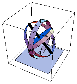
The model is run at T = 0.1 so that initial conditions are available for SolveFree.

In[26]:=

Out[26]=

10.3.4 Instantaneous Free Acceleration

To find the free acceleration of the gyroscope, one or more constraints must be dropped. The constraint that prevents rotation of the base, constraint 2, is dropped first. The rotor cannot precess in this state because the gimbal is still locked to the base, but the reaction torques applied to the base that accelerate the rotor can be measured.
No initial conditions are explicitly given. Initial guesses are taken from the default initial guesses that were set by the last run of SolveMech.

This drops the constraint that locks the base relative to the ground.

In[27]:=

This solves the FreeSystem object.

In[28]:=

The angular acceleration of the rotor is 1.0 in the Z direction. This corresponds to the 1.0 applied moment divided by the 1.0 moment of inertia about the Z axis.

In[29]:=

Out[29]=

There is no gyroscopic torque applied to the base by the Revolute5 constraint because the base has zero angular velocity at this instant.

In[30]:=

Out[30]=

To make this model a little more interesting, the base is given a nonzero angular velocity with the InitialCondition option for SolveFree. This induces gyroscopic torques in the base constraint. To be consistent with the constraints the Z components of the initial angular velocity of each body must be identical.

This solves the FreeSystem object with a new partial initial condition. The rest of the initial conditions are taken from LastSolve[].

In[31]:=

The angular acceleration of the rotor now has a component in the Y direction corresponding to the changing direction of the angular velocity vector.

In[32]:=

Out[32]=

Now there is a gyroscopic torque applied to the base by the Revolute5 constraint.

In[33]:=

Out[33]=

Now the FreeSystem is rebuilt with both the base and the gimbal unlocked. The same initial velocity for the base, gimbal, and rotor is used so that the gyroscope precesses.

This builds and solves the FreeSystem object with constraints 2 and 4 dropped.

In[34]:=

Without the constraint forces applied by constraint 4, the gimbal has an angular acceleration about its Y axis induced by the gyroscopic forces.

In[36]:=

Out[36]=

Again, there is no gyroscopic torque applied to the base by the Revolute5 constraint because the gimbal is free to rotate.

In[37]:=

Out[37]=

10.3.5 Gyroscopic Moments

Gyroscopic forces and moments modeled as per the example in Section 10.3.4 work well for single point analyses. However, if the time-domain free response is desired, such a modeling technique has a serious computational problem. While the rotor is spinning rapidly, the Euler parameters that represent the angular orientation of the rotor are changing sinusoidally and very rapidly. To numerically integrate such a system, the integrator must faithfully track very many periods of the sinusoidal Euler parameters to cover only a few periods of the motion of the more interesting parts of the gyroscope. If the period of the rotor's local rotation is much, much shorter than the period of interest, the integration becomes computationally infeasible.
The way around this problem is to introduce a special forcing function that mimics the gyroscopic torque of a spinning axially symmetric body and apply it to the rotor. This allows the rotor to be rotationally static.

A function to simulate gyroscopic moments.

GyroMoment has two important caveats attached to its use: the gyroscopic motion that it models is that of a body rotating about a principal axis of inertia and the two principle moments not associated with the axis of rotation must be equal. For most practical purposes, this means that the body is axially symmetric, and it is rotating about its axis of symmetry.
To demonstrate the use of GyroMoment, the gyroscope model that was presented in Section 10.3.3 is modified to remove the large angular velocity of the rotor and replace it with a GyroMoment load.

Here the gyroscopic moment simulation is added to the applied loads, the angular speed of the rotor body is reduced to zero, and the model is run at T = 0 so initial conditions are available to SetFree.

In[38]:=

Out[40]=

First, the constraint that locks the base to the ground is dropped and SolveFree is run with the Z direction angular velocity set to 1.

In[41]:=

The resulting angular velocities and accelerations are missing the large components that were due to the rotation of the rotor.

In[43]:=

Out[43]=

But the reaction at the base still reflects the gyroscopic torques.

In[44]:=

Out[44]=

This builds and solves the FreeSystem object with constraints 2 and 4 dropped.

In[45]:=

Without the rotation of the rotor, the angular accelerations of the rotor and gimbal are equal.

In[47]:=

Out[47]=

There is still no gyroscopic torque applied to the base when the gimbal is free to rotate.

In[48]:=

Out[48]=

The constraint reaction forces that result from using this method are identical to the reaction forces that result from the normal procedure, without the use of GyroMoment. The true values of alpha and omega for the simulated rotor are reproduced by the following calculation.

omegalocal is the local angular velocity vector that was passed to GyroMoment. Note that omegatrue and alphatrue match the angular velocity and acceleration components of the rotor in the previous analysis.

In[49]:=

Out[50]=

Out[51]=

The equations of motion that are produced by this method are essentially equivalent to the equations of motion without the spinning rotor simulation, with one important difference, these equations of motion can be easily integrated to obtain the time-domain motion of the entire gyroscope assembly without an overwhelming computational burden.

Undocumented Graphics Generation

10.4 Dynamic Motion Synthesis

This section covers the use of the SolveFree function to numerically integrate the equations of motion built by SetFree, which is done to find the time-domain dynamic motion of underconstrained systems. The FreeSystem objects that contain the equations of motion to be integrated are built using the same procedure that would be used if only the instantaneous free response was desired. Building such FreeSystem objects is covered in Sections 10.2 and 10.3.

10.4.1 Numerical Integration

Numerical integration with SolveFree.

There are several issues that are specifically associated with the numerical solution of the constrained equations of motion generated by MechanicalSystems. The equations of motion are a nonminimal differential-algebraic system of equations, that may or may not be linear in the highest-order terms.
One important issue is constraint violation. The equations of motion do not include the actual kinematic constraints, they only include the second time derivatives of the constraint equations. Because of this, small errors in the numerical integration of the equations of motion can accumulate into large violations of the kinematic constraints and their first derivatives. To deal with this problem, the equations can be algebraically reduced to a minimal set, but this is not generally possible with the type of constraints allowed by Mech. Alternatively, the numerical values of the dependent variables can be corrected as the integration progresses so as to continuously satisfy the constraints. This method is implemented in SolveFree.
Another issue is the transformation of angular velocity and acceleration in 3D models. If a model is built with angular coordinates (the Method -> Angular option in SetSymbols) the first and second derivatives of angular orientation are represented by the angular velocity, omega, and the angular acceleration, alpha. Unfortunately, omega is not the first derivative of the Euler parameters used to represent angular orientation. Thus, a coordinate transformation must occur at each time step to allow the Euler parameters to be integrated. SolveFree handles this transformation automatically, so models built in any coordinate system can be integrated.
The equations of motion are not necessarily linear in their highest-order terms, depending on the form of the applied loads. SolveFree automatically switches to an iterative solution method for nonlinear systems that allows them to be solved, albeit slowly.

Initialization Options

The only option that is concerned with the initialization of the integrator is the InitialCondition option. All other information needed to integrate the equations of motion is contained in the FreeSystem object. This option is most useful for repeatedly integrating the same FreeSystem with different sets of initial conditions without having to rerun SetFree.

An initialization option for SolveFree.

The list of rules required by InitialCondition is of the form returned by SolveMech. Using SolveMech to generate the initial conditions (which is essentially what is done by the default setting) guarantees that the initial conditions constitute a valid solution to the constraint equations. If initial conditions that do not satisfy the constraints are passed to SolveFree, the integration will proceed without difficulty, producing results that satisfy the differential equations of motion, but do not satisfy the kinematic constraints.
Note that a sufficient set of initial conditions for integrating a free acceleration system is returned by SolveMech[time, Solution -> Velocity], while a sufficient set of initial conditions for integrating an equilibrium velocity system is returned by SolveMech[time].

Integration Options

The following options are used to control the actual integration algorithm used by SolveFree. The default settings for these options are intended to produce reasonable results in the shortest possible time with a well-behaved system. Some tweaking may be required to get the best result from models with large accelerations or force discontinuities.

Options for controlling the SolveFree integrator.

More options for controlling the integrator.

The error estimation used by SolveFree makes an assumption that the approximate magnitude of each of the dependent variables is near to 1. While this assumption is certainly valid for Euler parameters that are between -1 and 1, and the 2D angular coordinate that has units of radians, it is up to the user to choose a system of units such that the linear dimensions of the model are not extremely large or small. While the error estimation routine does not look at the Lagrange multipliers (1, 2, ...) it is best to keep the units of force and mass such that the Lagrange multipliers are not extremely large or small, because other parts of the numerical solution method begin to produce significant errors when dealing with a wide range of numerical magnitudes.
When step size switching is enabled, SolveFree basically limits the maximum error in any dependent variable at a single time step to be less than the MaxError setting. If this is exceeded at a time step, the integrator backs up, halves the step size, and proceeds forward again. This error limit seems rather loose. If the same variable exhibited the maximum signed error at each time step, the cumulative error in that variable after 1000 time steps would be 0.1! In reality, the large errors occur at discrete points in the motion of a model, so the cumulative error is normally smaller.
The MaxError option can also be used to explicitly specify the error magnitude limits at which the time step size is halved, doubled, or when a corrective versus predictive step is taken. MathError -> {a, b, c} specifies that the time step size will be doubled if the sum of the maximum errors in the last four steps drops below c, it will be halved if the error in the current step goes above a, and an Adams-Moulton corrective step will be taken if the error is between a and b. Thus, MaxError -> {0.0001, 0.00001, 0.000001} is equivalent to the default setting of MaxError -> 0.0001.

Iterative Solution Options

The following options are used only to control the iterative solution block used for nonlinear models. These options have no effect on linear models.

Options for the Newton-Rhapson solution block in SolveFree.

Free acceleration models are always linear in the acceleration variables (X2dd, Y3dd, ...) but they may be nonlinear in the Lagrange multipliers (1, 2, ... ) if there are loads applied that are algebraically dependent on reaction forces, such as friction. Equilibrium velocity models can be nonlinear in the Lagrange multipliers, and they can also be nonlinear in velocity variables (X2d, Y3d, ...) if the applied loads are nonlinear functions of velocity. The second element in a FreeSystem object tells whether the model is linear or not. FreeSystem[...][[2]] returns True for nonlinear models.

Output Control Options

The following options are used to determine what data is returned by SolveFree, and what format is used to returned it.

Output options for SolveFree.

The StepSize data returned by the Diagnostics setting can be useful to help determine what should be chosen for a constant step size, if one is desired. The MaxError data included by Diagnostics is the measure of error used by the adaptive time step adjustment algorithm to decide when to change the step size.

10.4.2 Planar Example Mechanism

The following example uses the pendulum-on-a-rope model that was developed in Section 10.1. The pendulum is released from a constrained zero velocity position, that is not in static equilibrium, and the free response is found.
The spring force that was used to pull the pendulum off to one side is removed from the model, but gravity is retained. Also, nonzero moments of inertia are defined for each body, since the moments of inertia are relevant to the dynamics of the system, while they were not relevant to the equilibrium analysis.

This loads the Modeler2D package.

In[1]:=

Here are the three body objects, including the new inertia properties.

In[2]:=

The pendulum-on-a-rope model uses seven constraint objects. The constraints that fix the initial position of the model have been altered so that the pendulum may be released from an offset position.

Here are the constraints.

In[3]:=

Here is the gravitational load applied to the pendulum and slider.

In[4]:=

Now the model is run with SolveMech.

In[5]:=

Out[5]=

Here is the pendulum-on-a-rope model in its initial configuration.

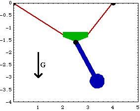
10.4.3 Free Response

To find the free acceleration of the pendulum, a FreeSystem object is built that contains a new set of equations of motion with constraints 5, 6, and 7 dropped from the model. Note that no initial conditions are yet available for the velocity of the bodies in the model. SetFree sets all of the initial velocities to zero if none are specified with the InitialCondition option.

This drops the constraints that lock the position of the pendulum. SetFree needs initial conditions for the velocity of each body. Since none are available zero is assumed.

In[6]:=

This integrates the FreeSystem object from T = 0 to T = 4.5, which is approximately a full period of the pendulum. The MakeRules option includes the velocity solution in the result.

In[7]:=

Here is a plot of the X coordinates of the slider and the pendulum.

In[8]:=

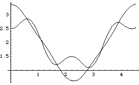
Out[8]=

Since the pendulum model is a conservative system, the sum of the kinetic and potential energy in the system should remain constant. This fact can be used to measure the accuracy of the numerical integrator.

A special output function.

The kinetic energy of each body is given by the BodyEnergy function, and the potential energy is simply the gravitational potential energy mass G altitude. The following plot shows that the numerical error in the integration has allowed the total energy of the model to increase by about 0.04% over 4.5 seconds.

Here is the total energy in the pendulum model.

In[9]:=

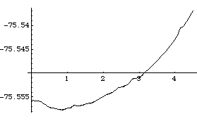
Out[9]=

Tightening the error budget by a factor of 100 by specifying the MaxError -> 0.000001 option for SolveFree will reduce the total energy rise to only 0.0007%, over the same time period, with an associated doubling of run time. Using the ConstraintCorrection -> True option, with the default error budget, will reduce the total energy rise to 0.002% with a slightly smaller increase in run time. In this case, either constraint correction or reducing step size (which is the result of decreasing the error budget) gives similar returns on computer time investment.
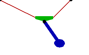
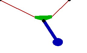
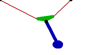
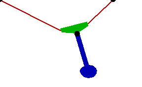
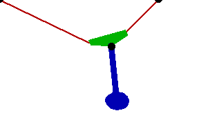
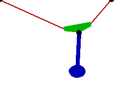
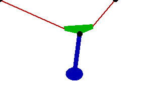
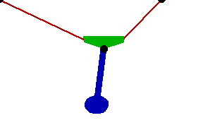
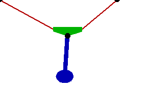
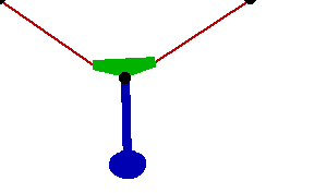
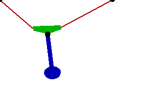
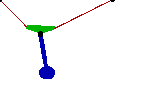
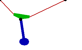
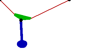
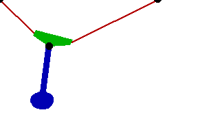
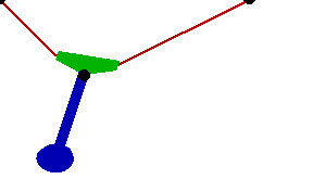
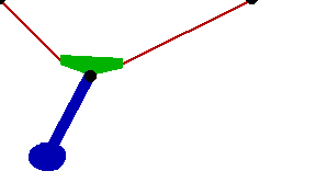
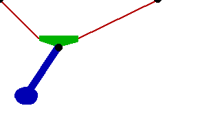
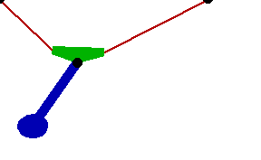
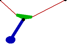
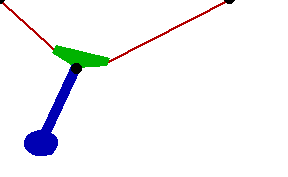
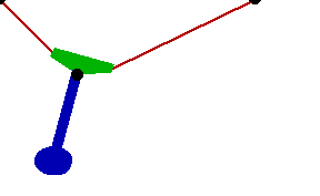
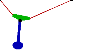
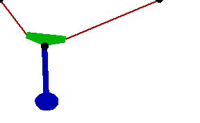
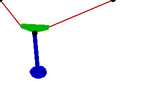
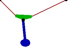
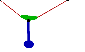
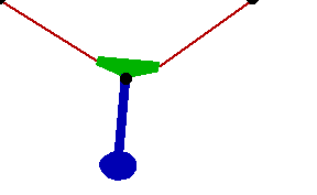
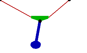
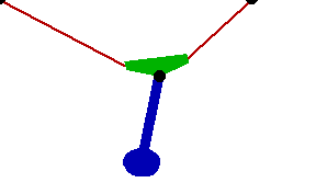
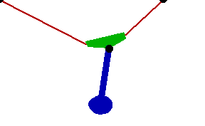
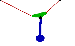
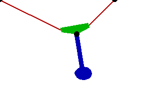
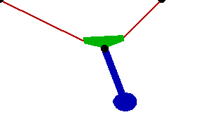
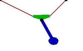
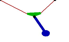
Changing the FitDegree setting can also affect the integration error. Setting FitDegree to Quadratic for this example will increase the net energy rise to 0.08%, while setting FitDegree to Quartic will reverse the sign of the error, changing the net energy rise to - 0.04%. Specifying a higher FitDegree setting often produces unexpected results because the automatic time step size adjustment works to counteract the higher degree setting. The integrator measures a smaller error in each step so it chooses a larger step size, resulting in the same net error.

Here is the pendulum-on-a-rope model at T = 1, 2, and 3 seconds.

Here is an animation of the pendulum-on-a-rope model.

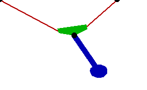
10.4.4 Gyroscopic Example

The following example integrates the motion of the gyroscope model that was presented in Section 10.3. The model uses the GyroMoment function, which was also presented in Section 10.3, to reduce the numerical burden of integrating the motion of the rotor. The angular local coordinate system is used, which requires SolveFree to use a coordinate transformation during the integration.

This loads the Modeler3D package and defines names for each of the body numbers.

In[10]:=

Here are the constraints, bodies, and loads for the gyroscope model.

In[16]:=

The model is run to prepare the initial conditions for SetFree. Note that the rotor has no angular velocity because it is modeled in the GyroMoment load.

In[20]:=

Out[20]=

10.4.5 Free Response

To find the unconstrained motion of the gyroscope, a FreeSystem object is built that contains a new set of equations of motion with constraints 2, 4, and 6 dropped from the model. Constraint 6, the constraint that locks the rotation of the rotor to that of the gimbal, is dropped in this simulation because the gross motion of the rotor results in some relative angular acceleration between these two bodies. If constraint 6 was not dropped, the model would represent an enforced constant angular velocity between the rotor and the gimbal, as if the rotor had a constant velocity motor attaching it to the gimbal.
The constant moment that was applied to the base is retained, so the model is expected to gain energy with the passage of time.

This drops the constraints that lock the three rotational axes of the gyroscope.

In[21]:=

This integrates the FreeSystem object from T = 0 to T = endt. The MakeRules option includes the velocity solution in the result.

In[22]:=

Here is a plot of the three components of the angular velocity of the gimbal. The Z component is simply oscillating about zero, so the applied torque is producing no net motion of the gimbal. The Y component, however, is consistently negative, so the gimbal is precessing in an oscillatory manner.

In[23]:=

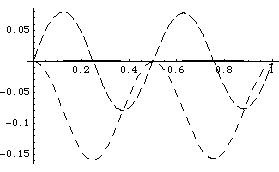
Out[23]=

Here is a plot of the rotation angle of the base.

In[24]:=

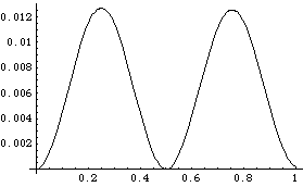
Out[24]=

Note that the Rotation function was not used in the preceding example to resolve the rotation angle of the base from the Euler parameters, but ProjectedAngle was used instead. This was done because the small numerical errors in the integration caused one of the Euler parameters to drift slightly above 1.0. The Euler parameters are not meaningful for absolute values greater than 1, so the Rotation function would return an error. The ProjectedAngle function uses vector algebra, instead of a mathematical identity, and it does not care if the values of the Euler parameters stray above 1.
Since the gyroscope model is a conservative system (if the applied moment is recognized as a conservative force) the sum of the kinetic and potential energy in the model should be constant. The potential energy stored by the constant applied moment is the work done by the gyroscope on the applied moment, which is the negative of the magnitude of the applied moment times the is rotation of the base. The following plot shows that the numerical error in the integration has allowed the total energy of the model to decrease by about 2% of the maximum kinetic energy over the integration period.

Here is the total energy in the gyroscope, including the energy stored in the constant applied moment.

In[25]:=

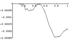
Out[25]=

This is near to the maximum kinetic energy of the body.

In[26]:=

Out[26]=

Tightening the error budget by a factor of 10 with MaxError -> 0.00001 will reduce the total energy rise to only 0.12% over the same period, with an associated increase in run time. Using the ConstraintCorrection -> True option, with the default error budget, will have virtually no effect on the error in the total energy. This is because the error stems from the deviation in the Euler parameters that are very close to 1, an error on which constraint correction has little effect. Using the FitDegree -> Quartic option, with the default error budget, will reduce the total energy rise to 0.71%, with only a small increase in run time.

10.4.6 Reducing Gyroscopic Models

There is one more technique that can be applied to 3D gyroscopic models to reduce their size and thereby reduce their run time. This technique can be very useful to models with more than one rotor.

A function for modifying an inertia tensor.

The restrictions that apply to the use of GyroFilter are identical to the restrictions that apply to the use of GyroMoment. The body represented by the inertia properties must be axially symmetric. The purpose of GyroFilter is to make it possible to add a zero-torque spinning body to a model without actually adding a body to the model at all. To demonstrate, the rotor body is deleted from the previously defined gyroscope model, and replaced with a special load and inertia properties on the gimbal. This time, the model is built in Euler coordinates, just to show that the results are the same.

Here is the gyroscope constraint set with the rotor deleted.

In[27]:=

Here is the body object for the gimbal. It now carries the inertia of what was the rotor with the component in the direction of the spin axis (the local X axis) of the rotor filtered out. Note the return from GyroFilter; the X component of the inertia is gone.

In[29]:=

Out[30]=

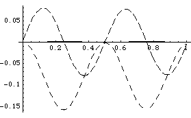
Here are the load objects. They are unchanged, except that GyroMoment uses the inertia option to explicitly specify the inertia properties. If this was not done, GyroMoment would pull the inertia properties from the body object that has previously had the X component filtered out.

In[31]:=

The model is now functionally equivalent to the previously defined model. The model can be integrated with SolveFree, after dropping constraints 2 and 4. Constraint 6 was previously dropped and is no longer part of the model.

The model is integrated from T = 0 to 1.

In[32]:=

Here is a plot of the angular velocity components of the gimbal. It is identical to the response of the previous model, with only two bodies required to create it.

In[35]:=

Out[35]=

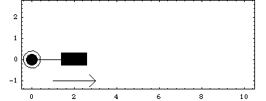
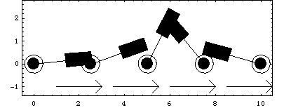
Undocumented Graphics Generation

10.5 Nonholonomic Systems

Nonholonomic systems, or systems that have a kinematic constraint that is an explicit function of velocity, are dealt with using the SetPath and SolvePath functions. SetPath is used to take a normally constrained kinematic model and replace one of its constraints with a constraint that is a function of mechanism velocities. SolvePath then integrates the resulting first-order system to obtain a time history of the motion of the mechanism.

10.5.1 Example Mechanism

The following planar example is probably one of the more common nonholonomic systems, a caster, such as a wheel on a shopping cart. The caster is modeled in two dimensions by viewing the caster from above, like looking down through the shopping cart. The steady state motion of a caster is for the wheel to trail directly behind the pivot point of the caster. What is modeled here is the motion of the caster when the direction of travel of the pivot is reversed. The caster swings out to one side of the pivot and then settles in behind the pivot again.
The wheel of the caster is modeled as a single nonholonomic constraint that constrains the direction of travel of the wheel to be parallel to the direction that the wheel is pointed. In vector algebra terms the velocity vector of the wheel is perpendicular to a vector through the wheel's axis of rotation. Normal Mech constraint functions can be used to model first-order relationships such as this by making at least one of the geometry specifications in the constraint a function of velocity.
Before the velocity constraint can be put in place by SetPath the model must be built in a normal kinematically constrained way. This requires a dummy constraint that will be replaced by SetPath later. The dummy constraint is a RotationLock1 constraint to lock the rotation of the caster relative to the ground. The other constraint in the model, constraint 1, simply constrains the pivot point of the caster to move steadily along the global X axis.

This loads the Modeler2D package.

In[1]:=

Here is a pair of constraints for the 2D caster model. The second constraint will be replaced with a velocity relationship by SetPath.

In[2]:=

The model is run just to make initial conditions available to SetPath.

In[5]:=

Here is the caster with zero initial angle.

10.5.2 Nonholonomic Constraints

The nonholonomic system solving functions.

This builds the PathSystem object. The second argument of the Orthogonal1 constraint is interpreted as a vector, in global coordinates, that is constrained to be orthogonal to the Vector on the caster.

In[6]:=

Out[6]=

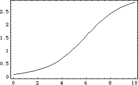
The InitialCondition option is used to give the caster a nonzero initial angle. Otherwise, it is simply pushed along in front of the pivot indefinitely, instead of swinging around behind the pivot as expected.

In[7]:=

Out[7]=

Here is a plot of the caster angle as a function of time. Note that T is equal to the X coordinate of the caster.

In[8]:=

Out[8]=

Here is a graphic of the caster at five positions between T = 1 and T = 10.

Undocumented Graphics Generation