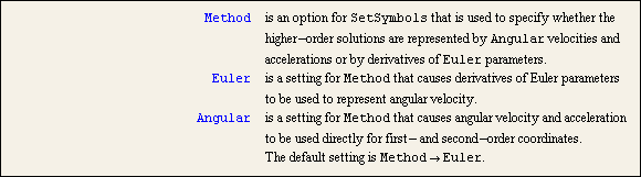
4.1 Velocity and Acceleration SolutionsMechanicalSystems calculates all velocities and accelerations with respect to the time variable (the symbol T by default). As was shown in Chapter 2, the use of the time variable in a model is optional, if the model is to be used to generate a location solution only. However, a model must have some explicit functional dependence on the time variable in order to have a nontrivial solution to the higher-order (velocity and acceleration) equations. 4.1.1 2D Example MechanismTo demonstrate the use of the Mech velocity and acceleration solutions, a 2D model is developed that can be measured. A 3D model is treated in the same manner as 2D with regard to higher-order solutions. The model is be a pull-rod and rocker rear suspension linkage for a car, consisting of three moving bodies: the chassis, the carrier, and the rocker. A real suspension linkage would have three more moving bodies: the upper and lower A-arms, and the pull-rod between the wheel carrier and the rocker.
The input to the model is the chassis moving vertically relative to the ground. This model could have been reduced in size by making the ground body the chassis, and simply moving the wheel carrier relative to the chassis, but the chosen method allows more flexibility and makes for better graphics.
The wheel carrier is attached to the chassis by two A-arms. These A-arms are not modeled as independent bodies because their function can be represented by a pair of relative distance constraints between the chassis and the wheel carrier.
The rocker pivots about an axis on the chassis and is attached to the wheel carrier by the pull-rod, a connecting link in tension. This pull-rod is also modeled with a relative distance constraint, not a separate body.
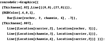
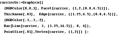
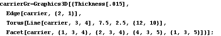
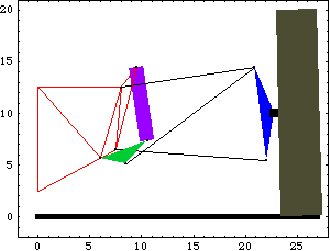
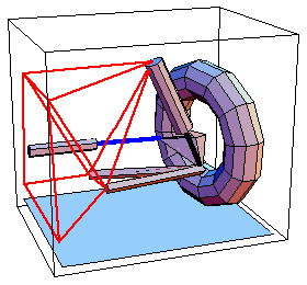
The shock absorber is connected between the other end of the rocker and the chassis. The damper is not actually part of the kinematic model at all, but the length of the damper as a function of wheel motion is a primary point of interest for any suspension linkage. Thus, the shock absorber exists only as a pair of mounting points on the chassis and the rocker, the separation of which can be measured as the car is bounced. Here is a graphic of the 2D pull-rod suspension model.
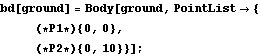
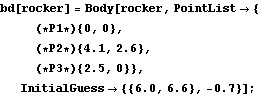
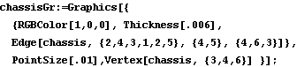
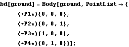
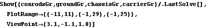
BodiesFour body objects are defined for the pull-rod suspension model. The ground body (body 1) requires two point definitions.
P1 is the origin of the ground body.
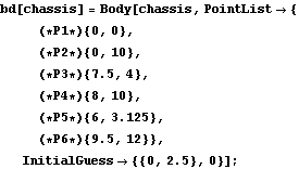
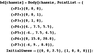
P2 is a point directly above the origin that defines a vertical translation line upon which the chassis slides.The chassis (body 2) requires six local point definitions.
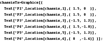
P1 is the local origin, which is a point at the bottom of the chassis.
P2 is a second point that, with P1, defines the vertical translation line of the chassis.
P3 is the pivot point of the lower A-arm.
P4 is the pivot point of the upper A-arm.
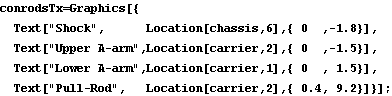
P5 is the pivot point of the rocker.
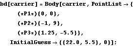
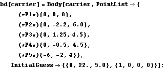
P6 is the upper mounting point of the shock absorber.The wheel carrier (body 3) requires three local point definitions.
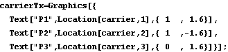
P1 is the local origin, which is the attachment point of the lower A-arm.
P2 is the attachment point of the upper A-arm and the pull-rod.
P3 is the bottom of the tire where the tire contacts the road.The rocker arm (body 4) requires three local point definitions.
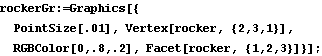
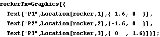
P1 is the local origin, which is the rotational axis of the rocker.
P2 is the lower attachment point of the shock absorber.
P3 is the attachment point of the connecting rod.Here are each of the bodies in the pull-rod model.
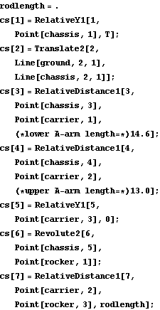
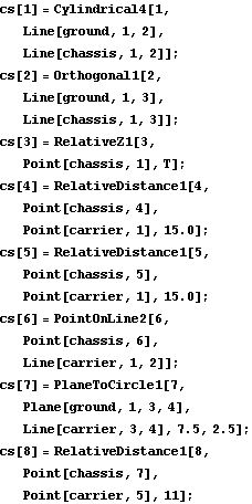
This loads the Modeler2D package and defines names for each of the bodies in the model. Here are the four body objects for the pull-rod model. The body objects must be incorporated into the current model with SetBodies. ConstraintsSeven constraints, one of which is a driving constraint with explicit dependence on time, are used to model the pull-rod suspension. A RelativeY1 constraint, used as a driving constraint, controls the vertical position of the chassis. This constraint is a driving constraint because it is functionally dependent on the time variable T.A Translate2 prismatic constraint controls the chassis rotation and horizontal position and allows the chassis to move only vertically relative to the ground.A RelativeDistance1 constraint models the upper A-arm.A RelativeDistance1 constraint models the lower A-arm.A RelativeY1 constraint forces the bottom of the tire to remain in contact with the ground.A Revolute2 constraint places the axis of the rocker arm.A RelativeDistance1 constraint models the pull-rod. The length of the pull-rod is specified by rodlength, which must be given a numerical value before Modeler2D attempts to find a solution.Here are the seven constraint objects for the pull-rod model. The constraint objects must be incorporated into the current model with SetConstraints. Note that the explicit symbol that is used to represent time in Modeler2D (T by default) may be changed. The SymbolBasis option for SetSymbols is a nested list of strings that determines the basis for all of the Global` symbols created by Modeler2D. Redefining the first element of SymbolBasis changes the symbol that is recognized as the time variable. SymbolBasis is the basis for all Modeler2D global symbols.
Out[20]= |  |
RuntimeBefore the model can be run, the symbol rodlength, which determines the length of the pull-rod, must be defined. Because of the presence of T in the driving constraint (constraint 1), the model can be run through its intended range of motion by varying T directly with the first argument to the SolveMech command. The way that this model is defined, the numerical value of T specifies the distance between the chassis and the ground. The symbol rodlength must be defined. Now the model is run at T = 2.5.
Out[22]= |  |
Here is the pull-rod suspension model at T = 2.5.
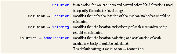
4.1.2 The Solution OptionWhen a Mech model is constructed with a functional dependence on the time variable T its time-domain motion is fully defined. Thus, nothing further needs to be done to generate velocity and acceleration solutions other than to ask for them. This is done with the Solution option for SolveMech. An option for SolveMech. The Modeler2D pull-rod suspension model defined in Section 4.1.1 is used to demonstrate the velocity and acceleration solutions. The Solution -> Velocity option causes SolveMech to calculate the location and velocity of each body in the model. This finds the location and velocity of each body at T = 3.0.
Out[23]= | 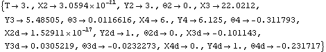 |
Mech creates a new set of symbols to represent the velocities and accelerations by appending a lowercase d or dd to each of the symbols that were used to represent body locations. Thus, while {X2, Y2} represents the location of the origin of body 2, {X2d, Y2d} represents the velocity of the origin of body 2.
Note that in this case, {X2d, Y2d} is equal to {0, 1}. This is expected since the driving constraint forces the height of the chassis to be T; therefore, its vertical velocity is equal to one.
The Solution -> Acceleration option causes SolveMech to calculate the location, velocity, and acceleration of each body in the model. This finds the location, velocity, and acceleration of each body at T = 3.0.
Out[24]= |  |
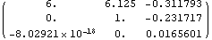
The location, velocity, and acceleration of the rocker (body 4) reflect the fact that its origin is stationary on the chassis, but its rotation is controlled in a nonlinear manner by the suspension linkage. Here is the rocker location, velocity, and acceleration. Out[25]//MatrixForm=
 |
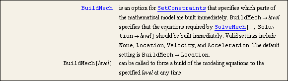
When SetConstraints is called to build the mathematical model, all of the expressions required for the velocity and acceleration solutions are not immediately built. Some parts of the mathematical model are built only when they are needed for the first time by SolveMech. Thus, the first time that SolveMech is called requesting a velocity or acceleration solution, it may take much longer to return a result than in any subsequent calls.
SetConstraints accepts the BuildMech option to force the modeling equations to be built to any level immediately, instead of waiting until they are needed. An option for SetConstraints. BuildMech can be used to build a model's velocity and acceleration equations before all of the symbolic parameters in the model have been defined, so that the parameters will remain variable in the model. If undefined parameters are present in a model, SolveMech cannot be called to seek a solution, but BuildMech can still build the required equations. Undocumented Graphics Generation4.1.3 3D Example MechanismA Modeler3D example model is developed to demonstrate the different angular velocity and acceleration formulations used by Modeler3D. This model is of a MacPherson strut automotive front suspension.
The model consists of only two moving bodies: the chassis and the wheel carrier. The wheel carrier is attached to the chassis by a lower A-arm, a MacPherson strut, and a steering tie rod that controls the steer angle of the wheel carrier. The A-arm, strut, and tie rod are not modeled as independent bodies in the model. They are each modeled as constraints that entirely represent the function they perform in the suspension. The input to the model is the chassis being moved vertically relative to the ground.
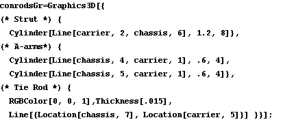
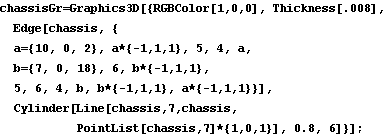
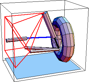
A MacPherson strut is attached to the chassis of a car by a ball joint, but it is attached to the wheel carrier in a cantilever fashion, not by another ball joint such as would be used in a more conventional double A-arm suspension. Thus, the MacPherson strut not only provides vertical support for the wheel carrier, it also provides the axis about which the wheel carrier pivots for steering. Since the strut cannot pivot with respect to the wheel carrier, it is modeled simply by forcing a ray on the wheel carrier to pass through a point on the chassis (the upper mounting point of the strut). This loads the Modeler3D package. Here is a 3D MacPherson strut front suspension model graphic.
BodiesThree body objects are defined for the MacPherson strut front suspension model. The ground body (body 1) requires four point definitions.
P1 is the origin of the ground body.
P2 is a point directly above P1 that is used in conjunction with P1 to define a vertical translation axis for the chassis.
P3 is a point on the X axis that is used with P1 to define a longitudinal axis that references the rotational orientation of the chassis.
P4 is a point on the Y axis that is used with P1 and P3 to define the horizontal plane of the ground upon which the tire rests.The chassis (body 2) requires seven local point definitions.
P1 is the origin of the chassis. This point lies at the center of the bottom of the chassis.
P2 is used in conjunction with P1 to define the vertical translation line of the chassis.
P3 is used with P1 to define a transverse axis on the chassis that is used to reference the rotational orientation of the chassis.
P4 and P5 are the two attachment points of the lower A-arm.
P6 is the upper mounting point of the MacPherson strut.
P7 is the attachment point of the steering tie rod. This point has a symbolic definition so that it can be moved in a transverse direction to steer the car.The wheel carrier (body 3) requires five local point definitions.
P1 is the local origin, which is the attachment point of the lower A-arm.
P2 is used with P1 to define the axis of the MacPherson strut on the carrier.
P3 is the center of the tire.
P4 is used with P3 to define the axis of the tire.
P5 is the attachment point of the steering tie rod on the wheel carrier.Names for each of the body numbers in the model are defined. Here are the three body objects used in the MacPherson strut model. The body objects are incorporated into the current model. ConstraintsEight constraints, including a driving constraint that is explicitly dependent on the time variable, are required to model the MacPherson strut front suspension. A Cylindrical4 constraint forces a vertical axis on the ground to be coincident with a vertical axis on the chassis, effectively allowing the chassis to slide up and down on a post.An Orthogonal1 constraint forces a longitudinal line on the ground to be orthogonal to a transverse line on the chassis. This constraint prevents the chassis from rotating about the vertical axis of rotation allowed by constraint 1.A RelativeZ1 constraint controls the vertical position of the chassis. This constraint is a function of the time variable T so it is the driving constraint.A RelativeDistance1 constraint models the front of the lower A-arm.A RelativeDistance1 constraint models the back of the lower A-arm.A PointOnLine2 constraint forces the axis of the MacPherson strut to pass through its upper mounting point on the chassis.A PlaneToCircle1 constraint forces the bottom of the tire to remain in contact with the ground. PlaneToCircle1 places the surface of a torus (or a circle) in contact with a plane.A RelativeDistance1 constraint models the steering tie rod.Here are the eight constraint objects for the MacPherson strut model. The constraints are incorporated into the current model. Note that the explicit symbol used to represent time in Modeler3D (T by default) may be changed. The SymbolBasis option for SetSymbols is a nested list of strings that determines the basis for all of the symbols created by Modeler3D in the Global` context. Changing the first element of SymbolBasis changes the symbol that is recognized as the time variable. SymbolBasis specifies the basis for Modeler3D automatic symbols.
Out[43]= |  |
RuntimeBecause of the presence of T in the driving constraint (constraint 3) the model can be run through its intended range of motion by varying T directly with the first argument to the SolveMech command. The way that this model is defined, the numerical value of T specifies the distance between the chassis and the ground. Now the model is run at T = 2.5.
Out[44]= | 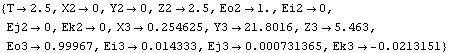 |
Here is the MacPherson strut front suspension image at T = 2.5.
4.1.4 3D Euler and Angular FormulationsVelocity and acceleration solutions are calculated in a 3D model in the same manner as in a 2D model. However, there are three options in a 3D model as to how the higher-order data is represented.
Since the angular orientation of Modeler3D bodies is specified by four Euler generalized parameters, {Eon, Ein, Ejn, Ekn}, one way of representing the angular velocity and acceleration of a body in 3-space is with the first and second derivatives of the Euler parameters, {Eond, ...} and {Eondd, ...}. Another more familiar way of representing angular velocity and acceleration is with the angular velocity and acceleration vectors, {omegaX, omegaY, omegaZ} and {alphaX, alphaY, alphaZ}, in either global coordinates or local coordinates attached to each individual body. Modeler3D can formulate the higher-order solutions in any of these representations, each of which requires that different sets of equations be built by the SetConstraints function. Which formulation is used is specified with the Method and Coordinates options for SetSymbols.

A system set-up function. The Method option for SetSymbols may also be used with Modeler2D to specify angular coordinates or a degenerate version of Euler coordinates, although the Euler coordinates are seldom used in 2D models. Specifying Method -> Euler in a Modeler2D model causes the angular orientation of each body to be represented by a pair of coordinates {Ejn, Ekn} = {cos( n), sin(n)} instead of a single coordinate, n. Velocity and acceleration are also represented by the coordinate pairs {Ejnd, Eknd} and {Ejndd, Ekndd}. The inclusion of this feature in Modeler2D is largely academic; specifying Method -> Euler causes four equations to be generated for each body, instead of only three, and usually slows down the solution phase. There are two advantages afforded by 2D degenerate Euler coordinates: no trigonometric functions are generated in the constraint expressions so all of the constraints are purely algebraic, and the second derivative of a 2D rotation matrix is very simple which leads to faster solutions in some dynamical systems. n), sin(n)} instead of a single coordinate, n. Velocity and acceleration are also represented by the coordinate pairs {Ejnd, Eknd} and {Ejndd, Ekndd}. The inclusion of this feature in Modeler2D is largely academic; specifying Method -> Euler causes four equations to be generated for each body, instead of only three, and usually slows down the solution phase. There are two advantages afforded by 2D degenerate Euler coordinates: no trigonometric functions are generated in the constraint expressions so all of the constraints are purely algebraic, and the second derivative of a 2D rotation matrix is very simple which leads to faster solutions in some dynamical systems. 2D/3DAn option for SetSymbols. 3DAn option for SetSymbols. The MacPherson strut front model defined in Section 4.1.3 is used to demonstrate the 3D velocity and acceleration solutions. The Solution -> Velocity option causes SolveMech to calculate the location and velocity of each body in the model. This finds the location and velocity of each body at T = 2.5.
Out[45]= | 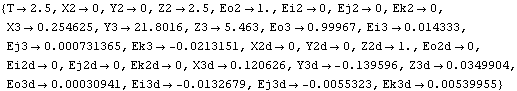 |
Note that the angular velocity of each body is returned in the form of derivatives of Euler parameters. This is because the constraint equations were built with all default options for SetSymbols. If the model is rebuilt with the Method -> Angular option for SetSymbols, the first derivatives of the Euler parameters will be replaced by angular velocities. This rebuilds the constraints with angular velocity formulation. Now find the velocity solution at T = 2.0.
Out[48]= | 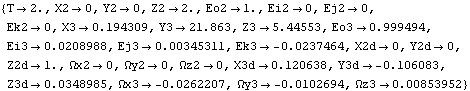 |
The angular velocity of the chassis in global coordinates is represented by the symbols { x2, y2, z2}. x2, y2, z2}.
The Solution -> Acceleration option causes SolveMech to calculate the location, velocity, and acceleration of each body in the model. Note that it takes more time to execute the following command the first time than it will on all subsequent executions. This is because the acceleration equations must be built the first time through. Now find the acceleration of the bodies at T = 2.0.
Out[49]= | 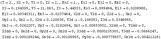 |
Since angular acceleration is the first derivative of angular velocity, the angular acceleration vector of the carrier, is represented by the derivatives of the angular velocity {x3d, y3d, z3d}.
The model is now rebuilt with the Coordinates -> Local option so that angular velocity is represented in local, instead of global, coordinates. This rebuilds the constraints with a local angular velocity formulation. Now find the velocity solution at T = 2.0.
Out[52]= | 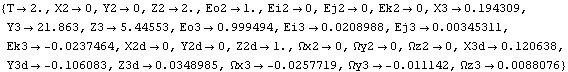 |
Note that the local angular velocity of body 3 is only slightly different from the global angular velocity. This is because the angular orientation of the wheel carrier is very close to being aligned with the global coordinate system. Undocumented Graphics Generation
|