|
Chapter 5
Finite Element Method
5.1 Introduction
This chapter introduces a number of functions for finite element analysis. First, one- and two-dimensional Lagrange and Hermite interpolation (shape) functions are introduced, and systematic approaches to generating these types of elements are discussed with many examples. You can design elements with desired features by manipulating terms in their basic functions. You can generate interpolation functions for many typical elements along with less conventional ones. Then you can create graphical representations of these interpolation functions. Finally, a number of useful auxiliary functions are also included.
You can solve many practical problems using a finite element procedure for plane elasticity problems. Since finite element analysis is an applied science, gaining experience in analysis is extremely crucial for the effectiveness of results. You can best acheive this by examining the intermediate steps of the analysis carefully and performing lots of calculations with various loading and meshing conditions. This chapter introduces functions for both the analysis and the intermediate steps of the analysis, along with graphical tools for clear representation of results. Mesh generation using the isoparametric formulation is also discussed with many examples.
5.2 One-Dimensional Shape Functions
5.2.1 General Remarks
With the package Element1D, you can compute the shape functions for one-dimensional Lagrangian- and Hermitian-type elements. You perform Hermite interpolation by fitting a curve to both an ordinate (field variable) and its slope (its derivative with respect to the local coordinate) at nodal points. The simplest Hermitian interpolation is between two nodal points at which the field variable and its derivative, with respect to the local coordinate, are known. Structural Mechanics contains the function HermiteElement1D for computing the Hermitian interpolation functions for one-dimensional elements. Lagrange interpolation is a special case of Hermite interpolation. In Lagrange interpolation, you obtain shape functions by fitting a curve for the field variables of a problem without concerning its derivatives.


5.2.2 Lagrange Elements
Generate the simplest Hermitian interpolation function,  , that is linear, one-dimensional, and has only two nodal points. The zero-order Hermitian interpolation functions are also known as Lagrange elements. Since for Lagrange elements do not require the continuity of the slope, the order of interpolation is zero, that is, n = 0. , that is linear, one-dimensional, and has only two nodal points. The zero-order Hermitian interpolation functions are also known as Lagrange elements. Since for Lagrange elements do not require the continuity of the slope, the order of interpolation is zero, that is, n = 0.
The length of the element is L and the coordinate is x in this example.
In[1]:=
In[2]:=
In[3]:=sfun0=HermiteElement1D[{0,L},0,x]
Out[3]=
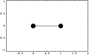
To plot the locations of the nodes of this simple element, you use the function ElementPlot.


Display two nodes at (x, y) = (0, 0) and (1, 0) with L = 1.
In[4]:=$DefaultFont={"Courier",7};
ElementPlot[{{{0,0},{1,0}}},PlotRange->{{-1,2},All},Frame->True];
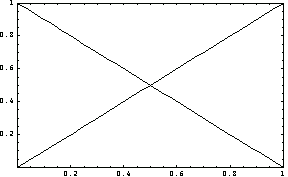
By definition, if the value of one of these interpolation functions is zero at a nodal point, the values of the other functions must be 1 at the same node. Plot these two interpolation functions to see if this condition is satisfied for L = 1 at x = 0 and x = L.
In[6]:=Plot[Evaluate[sfun0/.L->1],{x,0,1},PlotRange->{{0,1},{0,1}},Frame->True];
Similarly, you can easily generate higher-order interpolation functions for elements with more nodes. For example, compute the quadratic interpolation functions for equally spaced nodal points at (0, L/2, L).
In[7]:=sfun0=HermiteElement1D[{0,L/2,L},0,x]
Out[7]=
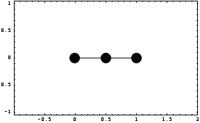
Display three nodes at (x, y) = (0, 0), (1/2, 0), and (1, 0) for L = 1. This shows the locations of the nodes.
In[8]:=ElementPlot[{{{0,0},{1/2,0},{1,0}}},
PlotRange->{{-1,2},All},
Frame->True];
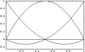
This shows these quadratic interpolation functions graphically.
In[9]:=Plot[Evaluate[sfun0/.L->1],{x,0,1},
PlotRange->{{0,1},{-0.25,1}},
Frame->True];
5.2.3 Hermite Elements
A  element provides inter-element continuity of the field variable (e.g., displacement, temperature, and so on) and its first derivatives (e.g., stress, heat flux, and so on) at the nodal points. In Lagrange-type elements, the solution for a field variable being approximated is continuous between elements; however, its derivatives are not necessarily continuous. Thus, only second-order partial differential equations can be approximated by Lagrange-type interpolation functions. In many cases, you might encounter higher-order differential equations. For example, in Euler-Bernoulli beam theory, the transverse deflection of the beam is governed by a fourth-order differential equation. Thus, the continuity of the first derivative of the solution (slope of the elastic curve in the beam problem) between elements is required since the slope is a primary variable, and the moment is the generalized force corresponding to this slope. element provides inter-element continuity of the field variable (e.g., displacement, temperature, and so on) and its first derivatives (e.g., stress, heat flux, and so on) at the nodal points. In Lagrange-type elements, the solution for a field variable being approximated is continuous between elements; however, its derivatives are not necessarily continuous. Thus, only second-order partial differential equations can be approximated by Lagrange-type interpolation functions. In many cases, you might encounter higher-order differential equations. For example, in Euler-Bernoulli beam theory, the transverse deflection of the beam is governed by a fourth-order differential equation. Thus, the continuity of the first derivative of the solution (slope of the elastic curve in the beam problem) between elements is required since the slope is a primary variable, and the moment is the generalized force corresponding to this slope.
You can easily obtain the simplest two-point Hermitian interpolation functions for  elements (that is, n = 1) as in the following example. The first two functions in the output correspond to continuity of the field variable (zero-order), and the last two are for the first-order continuity, that is, the derivatives, with respect to the local coordinate x, are continuous for these interpolation functions. elements (that is, n = 1) as in the following example. The first two functions in the output correspond to continuity of the field variable (zero-order), and the last two are for the first-order continuity, that is, the derivatives, with respect to the local coordinate x, are continuous for these interpolation functions.
In[10]:=sfun=HermiteElement1D[{0,L},1,x]
Out[10]=
The first function is unity at x = 0, and the second function is unity at x = L. All other functions are zero since the first two functions of the above output provide the inter-element continuity of the field variable, namely  continuity, while the last two are for the continuity of the first derivative of the field variable. continuity, while the last two are for the continuity of the first derivative of the field variable.
In[11]:=sfun/.x->0
Out[11]=
In[12]:=sfun/.x->L
Out[12]=
Similarly, the derivatives of the interpolation functions with respect to the coordinate x are unity at their corresponding nodal points.
In[13]:=D[sfun,x]/.x->0
Out[13]=
In[14]:=D[sfun,x]/.x->L
Out[14]=
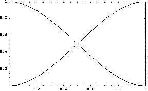
You clearly see the behavior of interpolation functions when you plot them. The length of the element L is equal to 1 in the following graphics. First, generate a plot for the inter-element continuity interpolation functions, which are given in the first two entries of the list sfun.
In[15]:=Plot[Evaluate[sfun[[1]]/.L->1],{x,0,1},
PlotRange->{{0,1},{0,1}},
Frame->True];
In[16]:=C1=sfun[[1]]/.L->1
Out[16]=
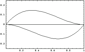
As expected (by definition), the first-order interpolation functions and their derivatives with respect to the local coordinate diminish at the nodal points. Here is the plot for the first-order interpolation functions.
In[17]:=Plot[Evaluate[sfun[[2]]/.L->1],{x,0,1},
PlotRange->{{0,1},{-0.25,0.25}},
Frame->True];
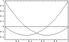
However, their derivatives with respect to x should behave as interpolation functions.
In[18]:=Plot[Evaluate[D[sfun[[2]],x]/.L->1],{x,0,1},
PlotRange->{{0,1},{-0.5,1}},
Frame->True];
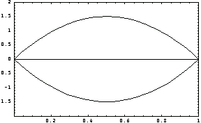
Similarly, the following plot shows that the derivatives of  interpolation functions at the nodal points are equal to zero. interpolation functions at the nodal points are equal to zero.
In[19]:=Plot[Evaluate[D[sfun[[1]],x]/.L->1],{x,0,1},
PlotRange->{{0,1},{-2,2}},
Frame->True];
5.3 Two-Dimensional Shape Functions
5.3.1 General Remarks
You can obtain the Lagrange shape functions for the rectangular elements whose nodes are placed in equally spaced intervals from the corresponding one-dimensional Lagrange shape functions. To do this, take the tensor product of one-dimensional shape functions in both the x and y coordinates.
Use one-dimensional shape functions to generate the Lagrange interpolation functions for the following four-node rectangular element. For an element with equally spaced nodes in two-dimensions, as shown in this example, you generate two-dimensional interpolation functions. In this example, the nodal points of the element are located at {1, 1}, {1, -1}, {-1, -1}, and {-1, 1}.
In[20]:=ElementPlot[{{{1,1},{1,-1},{-1,-1},{-1,1}}},
AspectRatio->1,
Axes->True,
PlotRange->{{-2,2},{-2,2}}];
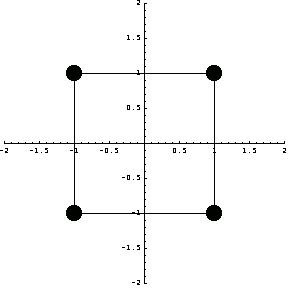
As previously, calculate the interpolation function of a one-dimensional two-node element in x using the function HermiteElement1D. The nodes of this element are placed at x = 0 and x = L, thus the element length is 2L.
In[21]:=HermiteElement1D[{-L,L},0,x]
Out[21]=
Since the nodal points are equally spaced in both the x and y coordinates, the tensor product of the shape functions in x and y gives four shape functions for the rectangular element. The length of the element in the x-direction is  , and the length of the other element is , and the length of the other element is  . Using the function HermiteElement, you first generate the linear Lagrange elements. Then, by taking the tensor product of the two sets of shape functions, you can compute the shape functions for the four-node rectangular element. . Using the function HermiteElement, you first generate the linear Lagrange elements. Then, by taking the tensor product of the two sets of shape functions, you can compute the shape functions for the four-node rectangular element.
In[22]:=sfun=Transpose[HermiteElement1D[{-L1,L1},0,x]].HermiteElement1D[{-L2,L2},0,y]
Out[22]=
You can easily verify that these are the desired interpolation functions by evaluating sfun at the nodal points of the rectangular element, namely, (  ), ( ), ( , ,  ), ( ), ( , ,  ), and ( ), and ( , ,  ). You can calculate the values of the interpolation functions sfun at x = ). You can calculate the values of the interpolation functions sfun at x =  and y = and y =  . .
In[23]:=sfun/.{x->L1,y->L2}
Out[23]=
Similarly, the point x  , y = , y =  satisfies the boundary conditions. satisfies the boundary conditions.
In[24]:=sfun/.{x->L1,y->-L2}
Out[24]=
The value of the interpolation function sfun at the point x =  , y = , y =  is the following. is the following.
In[25]:=sfun/.{x->-L1,y->L2}
Out[25]=
The value of the interpolation function sfun at the point x =  , y =- , y =-  is the following. is the following.
In[26]:=sfun/.{x->-L1,y->-L2}
Out[26]=
You can easily generalize this method for elements with more nodal points. Now generate interpolation functions for a nine-node element.
In[27]:=ElementPlot[{{{0,1},{1,1},{1,0},{1,-1},{0,-1},{-1,-1},{-1,0},{-1,1}},{0,0}},
AspectRatio->1,
Axes->True,
PlotRange->{{-2,2},{-2,2}},
Frame->True,
NodeColor->RGBColor[0,0,1]];
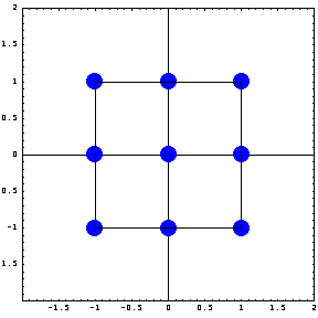
Similarly, here are the interpolation functions of the nine-node Lagrange element. The nodes in the x-direction are placed at x =  , x = 0, and x = , x = 0, and x =  while the the nodes in the y-direction are at y = while the the nodes in the y-direction are at y =  , y = 0, and y = , y = 0, and y =  . .
In[28]:=Transpose[HermiteElement1D[{-L1,0,L1},0,x]].HermiteElement1D[{-L2,0,L2},0,y]
Out[28]=
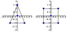
However, the situation becomes more complicated when you consider the elements whose nodes are not equally spaced in a grid. For example, you cannot generate the shape functions for triangular elements or the rectangular elements with irregular node locations by using the above tensor product approach. Here are two examples in which the interpolation functions cannot be generated.
In[29]:=p1=ElementPlot[{{{1,-1},{-1,-1},{0,3/2}},{0,0}},
AspectRatio->1,
Axes->True,
PlotRange->{{-2,2},{-2,2}},
NodeColor->RGBColor[0,0,1],
DisplayFunction->Identity];
In[30]:=p2=ElementPlot[{{{1,1},{1,-1},{-1,-1},{-1,1}},{0,0}},
AspectRatio->1,
Axes->True,
PlotRange->{{-2,2},{-2,2}},
NodeColor->RGBColor[0,0,1],
DisplayFunction->Identity];
In[31]:=
5.3.2 Triangular Elements
Use the functions TriangularCompleteness, RectangularCompleteness, and ShapeFunction2D to generate interpolation functions for triangular and general rectangular elements.


First, consider the triangular element with four nodal points and obtain a set of Lagrange-type shape functions, namely c = 0. Do not specify the minimum number of symmetric terms to be dropped from the full polynomial.
In[32]:=com=TriangularCompleteness[4,0,0];
com//TableForm
Out[33]//TableForm=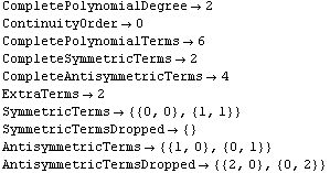
You can produce Pascal's triangle using the function PascalTriangle. Viewing this diagram and considering the output com, you can easily identify what terms to use in the shape functions and what terms to exclude.


In[34]:=
Out[34]=
In[35]:=
Out[35]=
In[36]:=TableForm[PascalTriangle[6,{x,y}],TableAlignments->Center]
Out[36]//TableForm=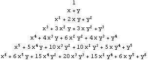
You compute the degrees of the terms in Pascal's triangle with the same function.
In[37]:=
Out[37]//MatrixForm=
This output tells you about the structure of the polynomial terms in the shape functions for this four-node triangular element. The term CompletePolynomialDegree->2 in the output list com implies that all the terms in the interpolation functions will consist of the terms of the second- and lower-degree polynomials.
In[38]:=1+(x+y)+(x+y)^2//Expand
Out[38]=
The second argument of the function TriangularCompleteness requires ContinuityOrder 0. CompleteSymmetricTerms 0. CompleteSymmetricTerms 2 tells you that the complete polynomial has two symmetric terms. Similarly, CompleteAntisymmetricTerms 2 tells you that the complete polynomial has two symmetric terms. Similarly, CompleteAntisymmetricTerms 4 indicates that there are four asymmetic terms in the interpolation functions. SymmetricTerms 4 indicates that there are four asymmetic terms in the interpolation functions. SymmetricTerms {{0, 0}, {1, 1}} will use both of the symmetric terms in the complete polynomial, namely the terms 1 and xy. SymmetricTermsDropped {{0, 0}, {1, 1}} will use both of the symmetric terms in the complete polynomial, namely the terms 1 and xy. SymmetricTermsDropped { } informs you that no symmetric term will be dropped. AntisymmetricTerms { } informs you that no symmetric term will be dropped. AntisymmetricTerms {{1, 0},{0, 1}} indicates that the only two asymmetric terms to be used are x and y. Finally, AntisymmetricTermsDropped {{1, 0},{0, 1}} indicates that the only two asymmetric terms to be used are x and y. Finally, AntisymmetricTermsDropped {{2, 0}, {0, 2}}} means that the terms {{2, 0}, {0, 2}}} means that the terms  and and  will be excluded in the interpolation functions. will be excluded in the interpolation functions.
The data provided in com are also called the completeness information for an element. Using the completeness data and the function ShapeFunction2D, you can systematically generate interpolation functions in two-dimensional elements.


Sometimes, the function ShapeFunctions2D is not able to generate a set of interpolation functions because the set of equations for computing the interpolation functions are singular. In these cases, ShapeFunctions2D will return zeros, as in this example.
In[39]:=ShapeFunctions2D[com,{{1,-1},{-1,-1},{0,3/2},{0,0}},{x,y}]
Out[39]=
This output simply means that the terms defined in com are not suitable to represent a set of interpolation functions for the given nodal points of the element. In other words, you cannot have a set of interpolation functions for this element in terms of xy, x, y, and a constant. At this point, you can try to use higher-order terms in your calculations. For example, change AntisymmetricTerms {{1, 0}, {0, 1}} in the output com to AntisymmetricTerms {{1, 0}, {0, 1}} in the output com to AntisymmetricTerms {{2, 0}, {0, 2}}; this allows the function ShapeFunctions2D to use the terms {{2, 0}, {0, 2}}; this allows the function ShapeFunctions2D to use the terms  and and  along with a constant and the cross term xy in constructing the desired interpolation functions. along with a constant and the cross term xy in constructing the desired interpolation functions.
In[40]:=com={CompletePolynomialDegree -> 2,
ContinuityOrder -> 0,
CompletePolynomialTerms -> 6,
CompleteSymmetricTerms -> 2,
CompleteAntisymmetricTerms -> 4,
ExtraTerms -> 2,
SymmetricTerms -> {{0, 0}, {1, 1}},
SymmetricTermsDropped -> {},
AntisymmetricTerms -> {{2, 0}, {0, 2}},
AntisymmetricTermsDropped -> {{1, 0}, {0, 1}}};
In[41]:=sfs=ShapeFunctions2D[com,{{1,-1},{-1,-1},{0,3/2},{0,0}},{x,y}]
Out[41]=
By expanding these functions, you can see the role of the terms used.
In[42]:=Expand[sfs]
Out[42]=
You can explore other possibilities to obtain different interpolation functions for the same element. For example, try to represent the shape functions in terms of a constant term,   x, and y. x, and y.
In[43]:=com={CompletePolynomialDegree -> 2,
ContinuityOrder -> 0,
CompletePolynomialTerms -> 6,
CompleteSymmetricTerms -> 2,
CompleteAntisymmetricTerms -> 4,
ExtraTerms -> 2,
SymmetricTerms -> {{0, 0}, {2, 2}},
SymmetricTermsDropped -> {},
AntisymmetricTerms -> {{1, 0}, {0, 1}},
AntisymmetricTermsDropped -> {{2, 0}, {0, 2}}};
In[44]:=fns=ShapeFunctions2D[com,{{1,-1},{-1,-1},{0,3/2},{0,0}},{x,y}]
Out[44]=
In[45]:=Expand[fns]
Out[45]=
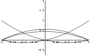
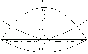
Now compare these interpolation functions by plotting sfs and fns along the x axis at y = -1. Note that two sets of interpolation functions present very different behaviors.
In[46]:=
In[47]:=
5.3.3 Rectangular Elements
Like TriangularCompleteness, you can use the function RectangularCompleteness to generate the neccessary information on the terms in the interpolation functions of a rectangular element.


Now compute the shape functions for the five-point rectangular element.
In[48]:=

Here are the coordinates of the nodal points of this element.
In[49]:=mm={{0,0},{1,1},{-1,1},{1,-1},{-1,-1}}
Out[49]=
Generate the element completeness information for the points.
In[50]:=sol4=RectangularCompleteness[5,0,0];
sol4//TableForm
Out[51]//TableForm=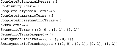
Here is how you generate the interpolation functions for this element.
In[52]:=sfun=ShapeFunctions2D[sol4,mm,{x,y}]
Out[52]=
Now draw the three-dimensional graphics of these five shape functions.
In[53]:=Table[Plot3D[sfun[[i]],{x,-1,1},{y,-1,1},
PlotRange->{{-2,2},{-2,2},All},
FaceGrids->{{0,0,-1}}],{i,1,5}];
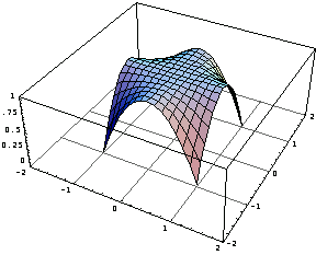
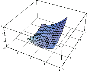
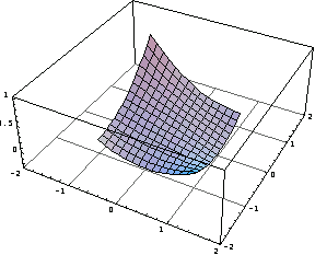
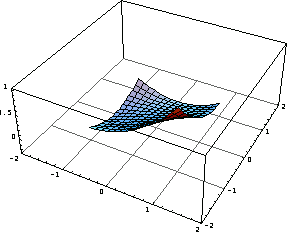
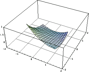
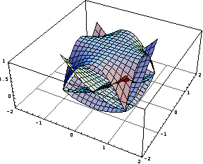
Superimpose the five graphs to display the basic idea behind the shape function concept.
In[54]:=Show[%];
5.3.4 Serendipity Elements
The serendipity elements are the rectangular elements with no interior nodes. You can obtain the shape functions of such elements using the functions RectangularCompleteness and ShapeFunctions2D. The main advantage of the serendipity elements is that since the internal nodes of the higher-order Lagrange elements do not contribute to the inter-element connectivity, the elimination of internal nodes results in reductions in the size of the element matrices.
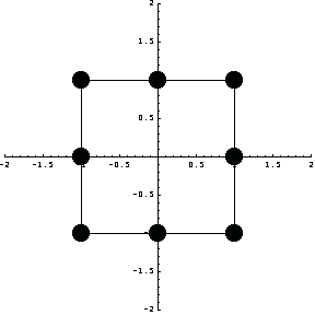
Now consider an eight-node  serendipity element with the following nodal points. serendipity element with the following nodal points.
In[55]:=pts={{0,1},{1,1},{1,0},{1,-1},{0,-1},{-1,-1},{-1,0},{-1,1}}
Out[55]=
Then you can plot the location of the nodal points of the element.
In[56]:=ElementPlot[{pts},
PlotRange->{{-2,2},{-2,2}},
Axes->True,
AspectRatio->1];
Here you can generate the completeness information for the element using the function RectangularCompleteness.
In[57]:=comp8=RectangularCompleteness[8,0,1];
comp8//TableForm
Out[58]//TableForm=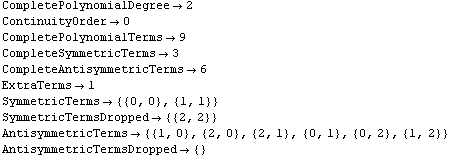
By using ShapeFunction along with the earlier completeness information, you can generate the interpolation functions for the element under consideration.
In[59]:=sfs=ShapeFunctions2D[comp8,pts,{x,y},{}];
sfs//TableForm
Out[60]//TableForm=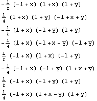
You can produce and superimpose the graphs of these functions.
In[61]:=Table[Plot3D[sfs[[i]],{x,-1,1},{y,-1,1},
PlotRange->{{-2,2},{-2,2},All},
FaceGrids->{{0,0,-1}},
DisplayFunction->Identity],{i,1,8} ];
In[62]:=Show[%,DisplayFunction->$DisplayFunction];
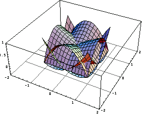
Now, as a more complicated example, you can produce the shape functions of a twelve-node serendipity element for the element with the following coordinates of the nodal points.
In[63]:=pts={{1/3,1},{1,1},{1,1/3},{1,-1/3},{1,-1},{1/3,-1},
{-1/3,-1},{-1,-1},{-1,-1/3},{-1,1/3},{-1,1},{-1/3,1}}
Out[63]=
You can see the locations of the nodes by using the function ElementPlot.
In[64]:=ElementPlot[{pts},
PlotRange->{{-2,2},{-2,2}},
Axes->True,
AspectRatio->1];
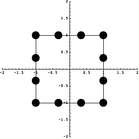
By dropping two symmetric terms from the appropriate complete polynomial, you can obtain the completeness information for this element.
In[65]:=comp12=RectangularCompleteness[12,0,2];
comp12//TableForm
Out[66]//TableForm=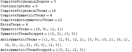
Using the function ShapeFunctions2D, it is simple to obtain the shape functions for this twelve-node serendipity element.
In[67]:=ShapeFunctions2D[comp12,pts,{x,y},{}]//TableForm
Out[67]//TableForm=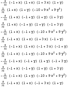
5.4 Plane Elasticity
5.4.1 General Remarks
This section solves a number of plane finite element problems to illustrate the functionality provided in Structural Mechanics. In addition to finite element analysis functions, many functions showing intermediate steps in a finite element analysis and producing graphical representation of results are included. You can use the functions StiffnessMatrix, ConstraintEquations, NaturalStateVariables, and EssentialStateVariables to calculate element stiffness matrices and to generate constraint equations and natural and essential variables. Using the functions FEModelPlot and DeformedMesh, you can generate a graphical representation of the mesh with nodal and element numbers, and the shape of the mesh after forces are applied.
The main function in the package PlaneElasticity is PlaneElasticityFEA.

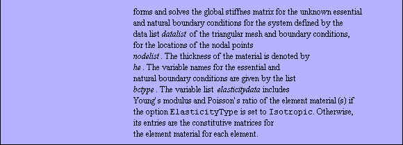

Options for the PlaneElasticityFEA function.
The format of the data list of the argument datalist for this function is as follows. Each nodal point is described by a list of four values:
 The first value is the number of a node. The first value is the number of a node.
 The second value is a list containing the element numbers that share this node. The second value is a list containing the element numbers that share this node.
 The third value is a list containing the constraints on the essential boundary conditions (displacements). The third value is a list containing the constraints on the essential boundary conditions (displacements).
 The last value contains the two components of the applied force (natural boundary condition) at this nodal point. The last value contains the two components of the applied force (natural boundary condition) at this nodal point.
5.4.2 Analysis Tools
Now, you examine the basic analysis tools available for finite element analysis while solving a simple problem. The list datalist in the following example represents a four-node, two-element finite element model. Nodes 1 and 4 are pinned in both the x- and y-directions, and two point forces are applied at these nodal points, one at node 2 in the x-direction with 160 po/2 magnitude and the other at node 3 with the same direction and magnitude. The nodes of element 1 are numbered as 1, 2, and 3, and the nodes of element 2 are 1, 3, and 4. In the list datalist, u denotes the essential type, while u[x] and u[y] are displacements in the x- and y-directions.
In[68]:=datalist= {
{1,{1,2},{u[x][1]==0,u[y][1]==0}, {0,0}},
{2,{1}, {}, {160 po/2,0}},
{3,{1,2},{}, {160 po/2,0}},
{4,{2}, {u[x][4]==0,u[y][4]==0}, {0,0}}
} ;
This representation of the model, boundary conditions, and applied forces is called datalist form. The coordinates of these nodal points are specified by the following list.
In[70]:=nodecoordinates={{0,0},{120,0},{120,160},{0,160}};
To view the locations of the nodes and elements, and to verify the model, you can draw the mesh of this model with the function FEModelPlot. The function FEModelPlot inherits the options of the Plot function in addition to its own specific options.


Options for the FEModelPlot function.
In[71]:=op=FEModelPlot[nodecoordinates, datalist,
PlotRange->{{-50,150},{-50,200}},
Axes->True];
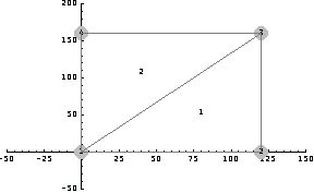
You can obtain the connectivity matrix of a model specified with datalist in datalist form using the function ConnectivityMatrix from its data list.


In[72]:=ConnectivityMatrix[datalist]
Out[72]=
PlaneElasticityFEA makes calls to a number of functions to calculate nodal forces and displacements. As the user, you can also call these functions. When the intermediate steps of a finite element analysis are of interest, you can adopt the functions in calculating the element stiffness matrix with the function StiffnessMatrix, the constraint equations with ConstraintEquations, and the symbols reserved for the natural and essential state variables NaturalStateVariables and EssentialStateVariables.


Options for the StiffnessMatrix function.
Compute the displacements and forces at the nodal points of this two-element plate model in plane stress. Make the thickness of the plate 0.036 inch and the distributed load po = 10.0 lb/inch. Name the coordinates and essential (displacement) and natural (force) boundary conditions {x, y} and {u, f}, respectively. The plate material is isotropic with Young's modulus E = 30   and Poisson's ratio and Poisson's ratio  = 0.25 for both elements. = 0.25 for both elements.
In[73]:=po=10.0; (* pressure field: constant in the force values *)
he=0.036; (* plate thickness *)
coordinates={x,y}; (* cartesian coordinates *)
bctypes={u,f} (* {essential, natural} *);
elasticitydata={{30 10^6,0.25},{30 10^6,0.25}}; (* Young's modulus, Poisson's ratio *)
In[78]:=sols1=PlaneElasticityFEA[datalist,bctypes,elasticitydata,nodecoordinates,he,
coordinates,ElasticityType->Isotropic,StressMode->PlaneStress];
In[79]:=sols1[[1]]
Out[79]=
To better view the solution, represent it in the format TableForm after sorting and flattening.
In[80]:=Flatten[Sort[sols1[1]]]//TableForm
Out[80]//TableForm=
In order to calculate the locations of the nodal points after the model was subjected to external forces, add the corresponding displacements to the nodes using the function DeformedMesh.


Now plot the deformed mesh with a large scaling factor, 2 ×  . .
In[81]:=FEModelPlot[DeformedMesh[sols1,nodecoordinates,2 10^4,{x,y},{u,f}],datalist,
PlotRange->All,ElementNumbers->False, NodeNumbers->False,
PlotStyle->RGBColor[0,0,1]];
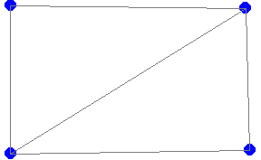
In[82]:=Show[op,%];
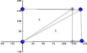
The output provides the forces and displacements at all of the nodal point of elements. While the displacement at the same nodal points of different elements are the same, the forces are not necessarily the same due to the fact that the equilibrium of the forces at a node is enforced. For example, at node 1 of the elements 1 and 2 you have calculated different values for the force component in the x-direction: f[x][1][1] -> 823.328 and f[x][1][2] -> -23.328. However, as expected, the displacement in either the x- or y-direction at point 3 are equal: u[x][3][1] -> -0.00101129 and u[x][3][2] -> -0.00101129.
5.4.3 Plane Stress versus Plane Strain
Here you can solve the same system with the plane strain assumption and compare the results.
In[83]:=sols2=PlaneElasticityFEA[datalist,bctypes,elasticitydata,nodecoordinates,he,coordinates,
ElasticityType->Isotropic,
StressMode->PlaneStrain];
Print the results under both assumptions side-by-side in table format. The first column of the following table corresponds to the solution with the plane stress assumption, StressMode->PlaneStress, and the second is with the plane strain assumption, StressMode->PlaneStrain.
In[84]:=Transpose[{Flatten[sols1],Flatten[sols2]}]//Chop//TableForm
Out[84]//TableForm=
The reaction forces in the x-direction in the plane stress case f[x][1][1] + f[x][1][2] = 800.00, and f[x][2][1] = 800.00, so the global force equlibrium in that direction is satisfied. From these data observe that the nodal forces in the plane strain case are larger than those in plane stress, whereas the nodal displacements for plane strain are less than those in plane stress.
5.4.4 Orthotropic Case
For anisotropic materials, you need to supply the function PlaneElasticityFEA with the material constants matrix C for each element. You can characterize an orthotropic material by four elasticity constants, and calculate the matrix C in the constitutive relations for both plane stress and plane strain cases using these four coefficients. Now compute the matrix C for both cases using the following data.
In[85]:=E1=31 10^6;
E2=2.7 10^6;
G12=0.75 10^6;
nu12=0.28;
Here is the matrix C for the plane stress case.
In[89]:=(* Plane Stress*)
nu21=nu12 E2/E1;
c11=E1/(1-nu12 nu21);
c22=E2/(1-nu12 nu21);
c12=nu21 c11;
c66=G12;
cmatrix1={{c11,c12,0},{c12,c22,0},{0,0,c66}};
MatrixForm[cmatrix1]
Out[96]//MatrixForm=
This is the matrix C for the plane strain case.
In[97]:=(* Plane Strain*)
nu21=nu12 E2/E1;
c11=E1(1-nu12)/(1-nu12-2nu12 nu21);
c22=E2(1-nu12 nu21)/((1+nu12)(1-nu12-2 nu12 nu21));
c12=E2 nu12/(1-nu12-2 nu12 nu21);
c66=G12;
cmatrix2={{c11,c12,0},{c12,c22,0},{0,0,c66}};
MatrixForm[cmatrix2]
Out[104]//MatrixForm=
Compute the forces and displacements at the nodal points of the mesh for both plane stress and plane strain and compare the results.
In[105]:=sols1=PlaneElasticityFEA[datalist,bctypes,{cmatrix1,cmatrix1},
nodecoordinates,he,coordinates,
ElasticityType->Anisotropic,
StressMode->PlaneStress];
In[106]:=sols2=PlaneElasticityFEA[datalist,bctypes,{cmatrix2,cmatrix2},
nodecoordinates,he,coordinates,
ElasticityType->Anisotropic,
StressMode->PlaneStrain];
In the following representation, the first column corresponds to plane stress, and the second column is for plane strain.
In[107]:=Transpose[{Flatten[sols1],Flatten[sols2]}]//Chop//TableForm
Out[107]//TableForm=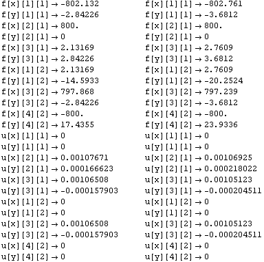
From this data, as in the previous example, observe that the nodal forces for plane strain are larger than those for plane stress, whereas the nodal displacements for plane strain are less than those for plane stress.
5.4.5 Four-Element Model
In general, the accuracy of a finite element analysis increases for models with more elements. However, there are some cases in which the accuracy may decrease with increasing element numbers. This section considers the same geometry with a four-element mode and examines the effect of the element numbers in a model. As for the two-element model, first prepare the arguments of the function PlaneElasticityFEA.
In[108]:=bctypes={u,f} (*{u: essential type BC, f: natural type BC } *);
nodecoordinates={{0,0},{120,0},{120,160},{0,160},{60.0,80.0}};
po=10.00; (* the numerical value of the applied force in datalist *)
datalist= {
{1,{1,4}, {u[x][1]==0,u[y][1]==0},{0,0}},
{2,{1,2}, {}, {160 po/2,0}},
{3,{2,3}, {}, {160 po/2,0}},
{4,{3,4}, {u[x][4]==0,u[y][4]==0},{0,0}},
{5,{1,2,3,4},{}, {0,0}}
} ;
elasticitydata={{30 10^6,.25},{30 10^6,.25},
{30 10^6,.25},{30 10^6,.25}}; (* Young's modulus, Poisson's ratio *)
coordinates={x,y};
he=.036; (* Plate thickness *)
Plot the mesh for the problem.
In[117]:=fe=FEModelPlot[nodecoordinates, datalist,
PlotRange->{{-50,150},{-50,200}},
Axes->True];
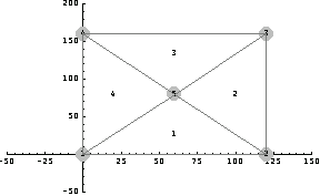
Again, determine the forces and the displacements at the nodal point of the model for plane strain and plane stress.
In[118]:=sols1=PlaneElasticityFEA[datalist,bctypes,
elasticitydata,nodecoordinates,he,coordinates,
ElasticityType->Isotropic,
StressMode->PlaneStress];
In[119]:=sols2=PlaneElasticityFEA[datalist,bctypes,
elasticitydata,nodecoordinates,he,coordinates,
ElasticityType->Isotropic,
StressMode->PlaneStrain];
Here is the table representation of the two results.
In[120]:=Transpose[{Flatten[sols1],Flatten[sols2]}]//Chop//TableForm
Out[120]//TableForm=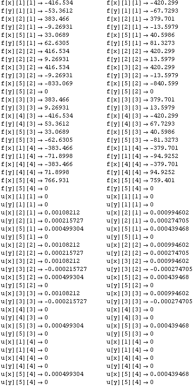
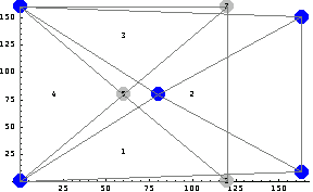
The x-component of the displacement at node 2 in the four-element model for the plane strain case, 0.001082 unit, is slightly higher than that in the two-element model, 0.001057 unit. The y-component of the displacement at the same node in the four-element model for plane stress case, 0.002157 unit, is higher than that in the two-element model, 0.0002569 unit. This observation is in accordance with the general belief that the models with fewer elements usually tend to be stiffer.
Plot the deformed meshes for both cases with a large scaling factor, 4 ×  . First, generate the deformed plot for the plane stress case. . First, generate the deformed plot for the plane stress case.
In[121]:=
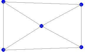
The original mesh and the deformed mesh are shown together.
In[122]:=
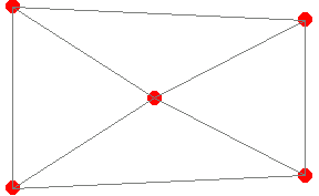
Here is the deformed mesh for plane strain.
In[123]:=
In[124]:=
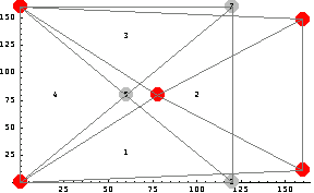
Here compare the deformations obtained under the plane stress and plane strain assumptions.
In[125]:=
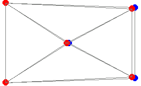
This plot reveals that the deflections for the plane stress case is greater than that for the plane strain case.
5.4.6 Mesh Generation: Triangulation
In previous examples, the analysis domain is triangulated by the user when forming the data list datalist. Using the function PolygonTriangulate, a domain specified by a polygon can be partitioned into triangles.


Triangulate the domain defined by the following list of points using the function PolygonTriangulate.
In[126]:=pts={{0.799109, 0.201991}, {0.799109, 0.798019},
{0.005076, 0.791397}, {0.005076, 0.208613},
{0.209724, 0.208613}, {0.209724, 0.579475},
{0.594461, 0.586098}, {0.598554, 0.201991}};
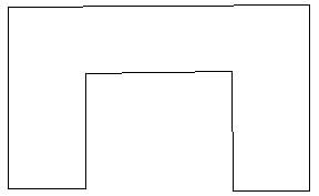
This is how the cross section looks before triangulation.
In[127]:=ori=Show[Graphics[Line[Append[pts,pts[[1]] ]]]];
In[128]:=con=PolygonTriangulate[pts]
Out[128]=
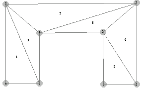
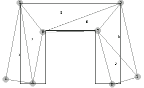
A six-triangle partition results. The vertices of the first triangle are formed by the nodal points 3, 4, 5, and so on. Using the function MeshPlot from the package TriangulatePolygon, you can generate a graphic representation of this triangulation. The function MeshPlot inherits its options from the Plot function.


In[129]:=MeshPlot[pts,con,PlotRange->All];
Using the function ConnectivityMatrix in a reverse manner, you can generate the data list output showing how the nodes are connected to the elements.
In[130]:=dl=ConnectivityMatrix[Table[{i,con[[i]]},{i,1,Length[con]}]]
Out[130]=
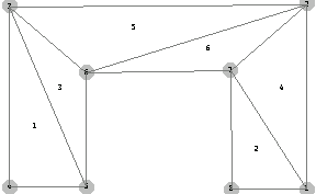
This result shows that node 1 is shared by elements 2 and 4, node 2 is shared by elements 4, 5, and 6, and so on.
You can obtain the same mesh using FEModelPlot where the list dl represents the data list of a finite element model. Note that for an analysis, you need to have the boundary conditions and the applied forces in this data list.
In[131]:=FEModelPlot[pts,dl];
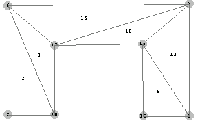
Both nodes and elements can be labeled in any way you wish. For example, you can number the nodes with even numbers and the elements with consecutive multiples of three.
In[132]:=ptsno=Table[{2 i, pts[[i]]},{i,1,Length[pts]}];
In[133]:=connect=Table[{3 i,con[[i]]},{i,1,Length[con]}];
The following plot presents the numbering of the mesh.
In[134]:=MeshPlot[ptsno,connect,PlotRange->All];
5.4.7 Channel Section Model
This section considers a channel section subjected to a force couple. First generate a triangular mesh for the structure. Then obtain the forces and displacements at the nodal points for the cases of plane strain and plane stress. Lastly, compare the two results.
Here are the coordinates of the nodal points.
In[135]:=pts=1000 {{0.79, 0.20}, {0.79, 0.79},
{0.00, 0.79}, {0.00, 0.20},
{0.20, 0.20}, {0.20, 0.59},
{0.59, 0.59}, {0.59, 0.20}};
Now generate the triangular mesh, pts, and the connectivity matrix, dl, for this model.
In[136]:=con=PolygonTriangulate[pts]
Out[136]=
In[137]:=dl=ConnectivityMatrix[Table[{i,con[[i]]},{i,1,Length[con]}]]
Out[137]=
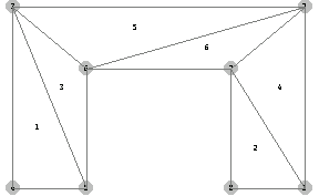
The following plot presents the mesh dl with nodal points and element numbers.
In[138]:=om=FEModelPlot[pts,dl,PlotRange->All];
Apply two units of force at nodes 1 and 4 in the x-direction and fix the model at nodes 2 and 3 in the x- and y-directions: u[x][2] = 0, u[y][2] = 0, and u[x][3] = 0, u[y][3] = 0. The data list for these modes is generated as follows.
In[139]:=datalist=
{{1, {2, 4}, {}, {1,0} },
{2, {4, 5, 6},{u[x][2]==0,u[y][2]==0},{0,0} },
{3, {1, 3, 5},{u[x][3]==0,u[y][3]==0},{0,0} },
{4, {1}, {}, {-1,0}},
{5, {1, 3}, {}, {0,0} },
{6, {3, 5, 6},{}, {0,0} },
{7, {2, 4, 6},{}, {0,0} },
{8, {2}, {}, {0,0} }};
bctypes={u,f} (* {u: essential type BC, f: natural type BC } *);
nodecoordinates = 1000 {{0.79, 0.20}, {0.79, 0.79},
{0.00, 0.79}, {0.00, 0.20},
{0.20, 0.20}, {0.20, 0.59},
{0.59, 0.59}, {0.59, 0.20}};
Here are the elasticity properties of the channel section material. The material is isotropic, and he is the section thickness.
In[143]:=elasticitydata=Table[{30. 10.^6,.25},{6}]; (* Young's modulus, Poisson's ratio *)
coordinates={x,y};
he=.01; (* Plate thickness *)
First, solve the model under the plane strain assumption. In this model, the plane strain approach is more realistic since the length of the section is much larger than the other dimensions of the cross section.
In[147]:=sols1=PlaneElasticityFEA[datalist,bctypes,
elasticitydata,nodecoordinates,he,coordinates,
ElasticityType->Isotropic,
StressMode->PlaneStrain];
Now, solve the same problem with the plane stress assumption.
In[148]:=sols2=PlaneElasticityFEA[ datalist,bctypes,
elasticitydata,nodecoordinates,he,coordinates,
ElasticityType->Isotropic,
StressMode->PlaneStress];
In the following, compare the plane strain (first column) and the plane stress (second column) approaches.
In[149]:=Transpose[{Flatten[sols1],Flatten[sols2]}]//Chop//TableForm
Out[149]//TableForm=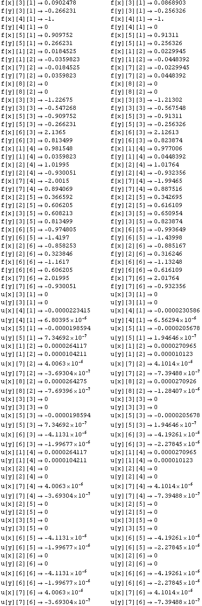
As in the example in Section 5.4.3, the nodal forces obtained under the plane strain assumption are larger than those for the plane stress case, whereas the nodal displacements for the plane stress case are less than those for plane strain case. Since the magnitude of the displacements are very small compared to that of the coordinates of the nodal points, you need to scale the displacements so that their effect can be visually presented. Take the value of this factor 5 ×  in the following representation. in the following representation.
In[150]:=do=FEModelPlot[DeformedMesh[sols1,nodecoordinates,5. 10^6,{x,y},{u,f}],datalist,PlotRange->All];
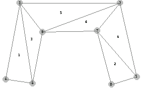
Superimpose the original mesh and the deformed mesh with upscaled displacements by a factor of 5 ×  . .
In[151]:=
5.4.8 Cantilever Beam Model
This section focuses on the analysis of a cantilever beam subjected to an edge load at the free end. It assumes that the material of the beam is isotropic, and that the stress mode of this analysis is plane stress. In this analysis, you can use the different finite element meshes consisting of linear triangular elements, and the triangulation scheme introduced in Structural Mechanics. After discussing the shortcomings of this type of triangulation, this section gives a simple method of producing a more regular mesh and carries out the analysis with the regular mesh. Finally, a finer regular mesh is considered and the results are compared with the analytical solution for the cantilever beam.
Triangular Mesh
Generate the mesh for a 10-inch cantilever beam with a rectangular 2 × 1 cross section using the triangulation function PolygonTriangulate. First, make sure that the nodal points are placed in the counterclockwise direction.
In[152]:=ptsn={{0,0},{10/3,0},{20/3,0},{10,0},{10,2},{20/3,2},{10/3,2},{0,2}}
Out[152]=
Then calculate a triangulation for these nodes.
In[153]:=con=PolygonTriangulate[ptsn]
Out[153]=
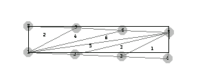
This shows the triangulation con generated with the triangulation function PolygonTriangulate.
In[154]:=MeshPlot[ptsn,con,
PlotRange->All,
AspectRatio->.2];

You could generate a different mesh that would partition the analysis domain into more regular triangles with symmetries.
Generate the connectivity matrix of this triangulation.
In[155]:=ConnectivityMatrix[Table[{i,con[[i]]},{i,1,Length[con]}]]
Out[155]=
In the data list datalist, specify the boundary conditions for specified forces and displacements. Fix the cantilever beam at nodes 1 and 8 in the x- and y-directions. Apply two point forces of 150 lb. at the free end of the beam, that is, nodes 4 and 5 in the negative y-direction. The list datalist contains the connectivity information of the model and the boundary conditions.
In[156]:=datalist={
{1, {2,4,5,6}, {u[x][1]==0,u[y][1]==0},{0, 0}},
{2, {3,5}, {}, {0, 0}},
{3, {1,3}, {}, {0, 0}},
{4, {1}, {}, {0, -150}},
{5, {1,3,5,6}, {}, {0, -150}},
{6, {4,6}, {}, {0, 0}},
{7, {2,4}, {}, {0, 0}},
{8, {2}, {u[x][8]==0,u[y][8]==0},{0, 0}}};
In the following, you can define the variable names for the boundary types, the elasticity coefficients of the isotropic beam material, and the beam thickness.
In[157]:=bctypes={u,f} (* {u: essential type BC, f: natural type BC } *);
nodecoordinates=ptsn;
elasticitydata=Table[{30. 10.^6,.25},{6}]; (* Young's modulus, Poisson's ratio *)
coordinates={x,y};
he=1.00; (* Plate thickness *)
Using the function PlaneElasticityFEA, you can calculate the forces and the displacement at the nodal points for the plane stress mode.
In[162]:=sols2=PlaneElasticityFEA[ datalist,bctypes,elasticitydata, nodecoordinates,he,coordinates,
ElasticityType->Isotropic,
StressMode->PlaneStress];
You intuitively know that the maximum displacement is realized at the free end of the beam at nodes 4 and 5.
In[163]:=u[y][4][1]/.sols2
Out[163]=
In[164]:=
Out[164]=
In[165]:=u[y][5][1]/.sols2
Out[165]=
Then you can compute the exact value of this displacement using the analytical solution for the cantilever beam.
In[166]:=pf=-2 150;
E1=30 10^6;
nu=.25;
L=10.;
I1=2/3;
exactdef=(pf L^3/(3 E1 I1)) (1+3.(1+nu)/L^2)
Out[171]=
Here is the ratio of the exact solution to the finite element solution obtained earlier at node 4.
In[172]:=exactdef/u[y][4][1]/.sols2
Out[172]=
The exact displacement is over 10 times larger than the approximate one. The reason for this large error, as will become clear in the next two examples, is due to the sparse elements and irregular meshing.
Using the function DeformedMesh, you can draw the deformed mesh with magnified displacements at a factor of 1000.
In[173]:=fe2=FEModelPlot[DeformedMesh[sols2,nodecoordinates,10^3,{x,y},{u,f}], datalist,PlotRange->All,AspectRatio->.2];

In[174]:=pl1=Show[fe2,Graphics[Line[Append[ptsn,ptsn[[1]]]]],
AspectRatio->.4,PlotRange->{{-2,12},{-2,4}}];
Regular Mesh
In the previous example, an irregular triangulation generated by PolygonTriangulate was used as the mesh. The tip displacement was about 10 times larger than the linear theory predicted. Now focus on the regularity of the mesh and study the effect of the grid structure on finite element results. Without changing the number of elements in the model, you can use a regular grid with 4 nodes in the x-direction, and 2 points in the y-direction as the mesh. The nodes are equally spaced in their respective directions.
In[175]:=n1=4;
n2=2;
The following Mathematica lines generate the connectivity information of the model.
In[177]:=nds=Table[{ {i+(j-1) n1,i + (j-1) n1 +1,i+1+j n1},
{i+(j-1) n1,i+j n1,i+1+j n1}},
{i,1,n1-1},
{j,1,n2-1}];
pt=Partition[Flatten[nds],3]
Out[179]=
Number the nodes from 1 to 6.
In[180]:=con=(k=0;Map[{++k,#}&,pt])
Out[180]=
Next compute locations of nodes 1 to 6.
In[181]:=xo=0;
yo=0;
dx=10/(n1-1);
dy=2/(n2-1);
pts=Partition[Flatten[Table[{ xo + (i-1) dx, yo + (j-1) dy},
{j,1,n2},{i,1,n1}]],2]
Out[185]=
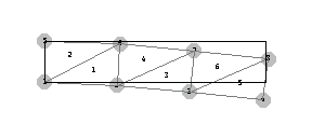
These connectivity data and nodal points result in the following mesh.
In[186]:=MeshPlot[pts,con,PlotRange->All,AspectRatio->.2,Axes->True];

Here is the connectivity matrix for this mesh.
In[187]:=con1=ConnectivityMatrix[con]
Out[187]=
From this connectivity matrix and the boundary conditions, you can construct the data list and the other arguments of the function PlaneElasticityFEA for the new model.
In[188]:=datalist={
{1, {1, 2}, {u[x][1]==0,u[y][1]==0},{0, 0}},
{2, {1, 3, 4}, {}, {0, 0}},
{3, {3, 5, 6}, {}, {0, 0}},
{4, {5}, {}, {0,-150}},
{5, {2}, {u[x][5]==0,u[y][5]==0},{0, 0}},
{6, {1, 2, 4}, {}, {0, 0}},
{7, {3, 4, 6}, {}, {0, 0}},
{8, {5, 6}, {}, {0,-150}}};
In[189]:=bctypes={u,f} (* {u: essential type BC, f: natural type BC } *);
nodecoordinates=pts;
elasticitydata=Table[{30. 10.^6,.25},{6}]; (* Young's modulus, Poisson's ratio *)
coordinates={x,y};
he=1.00; (* Plate thickness *)
In[195]:=sols1=PlaneElasticityFEA[datalist,bctypes,elasticitydata,nodecoordinates,he,
coordinates,
ElasticityType->Isotropic,
StressMode->PlaneStress];
Here are the endpoint displacements at the same nodal point as in the previous mesh.
In[196]:=u[y][4][5]/.sols1
Out[196]=
In[197]:=u[y][8][5]/.sols1
Out[197]=
This improves the accuracy of the endpoint displacements, but the true displacement to calculated displacement ratio is still high. As shown in the following, the ratio is almost 6. However, this example clearly demonstrates the positive effect of the regular mesh on the accuracy of results. In the next example, you can use a refined model in order to study its effect further.
In[198]:=exactdef/u[y][4][5]/.sols1
Out[198]=
Here is how the deflected beam looks with a magnification factor of  . .
In[199]:=fe=FEModelPlot[DeformedMesh[sols1,nodecoordinates,10^3,{x,y},{u,f}],datalist, PlotRange->All,AspectRatio->.2];

In[200]:=pl2=Show[fe,Graphics[Line[Append[ptsn,ptsn[[1]] ]]],
AspectRatio->.4,PlotRange->{{-2,12},{-2,4}}];
Finer Regular Mesh
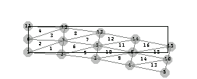
Now you can further refine the mesh for the cantilever beam problem to study the effect of the number of elements on the accuracy of approximated endpoint displacements. This grid will have five nodes in the x-direction, and 3 points in the y-direction. The nodes are equally spaced in their respective directions. As in the previous example, first produce the mesh.
In[201]:=n1=5;
n2=3;
In[203]:=nds=Table[{{i+(j-1)n1,i+(j-1)n1+1,i+1+j n1},
{i+(j-1)n1,i+j n1,i+1+j n1} },
{i,1,n1-1},
{j,1,n2-1}];
In[204]:=pt=Partition[Flatten[nds],3];
con=(k=0;Map[{++k,#}&,pt]);
xo=0;
yo=0;
dx=10/(n1-1);dy=2/(n2-1);
In[209]:=nodecoordinates=Partition[Flatten[Table[{xo+(i-1)dx,yo+(j-1)dy},{j,1,n2},
{i,1,n1}]],2];
This produces the mesh that is specified by the nodal points pts, the meshing information con, and a number of MeshPlot options.
In[210]:=

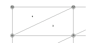
By setting the plot range option PlotRange->{{0,3},{0,2.5}}, you can closely view portions of elements 3 and 4 on the upper-left corner of the mesh.
In[211]:=MeshPlot[nodecoordinates,con,
PlotRange->{{-0.5,3},{.75,2.25}},
AspectRatio->.5,
Axes->False];
Generate the connectivity matrix of this mesh from the meshing information con using the function ConnectivityMatrix.
In[212]:=con1=ConnectivityMatrix[con];
Add { } and {0, 0} for the boundary conditions and the applied forces to the list con1.
In[213]:=Map[{#[[1]],#[[2]],{},{0,0}}&,con1]//MatrixForm
Out[213]//MatrixForm=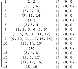
Now edit the output of this line to include the boundary conditions (u[x][1] = 0, u[y][1] = 0, u[x][6] = 0, u[y][6] = 0, u[x][11] = 0, and u[y][11] = 0), and the applied forces {0, -75} at nodal point 5, {0, -150} at nodal point 10, and {0, -75} at nodal point 15.
In[214]:=datalist=
{ {1, {1,2}, {u[x][1]==0,u[y][1]==0}, {0, 0}},
{2, {1,5,6}, {}, {0, 0}},
{3, {5,9,10}, {}, {0, 0}},
{4, {9,13,14}, {}, {0, 0}},
{5, {13}, {}, {0, -75}},
{6, {2,3,4}, {u[x][6]==0,u[y][6]==0}, {0, 0}},
{7, {1,2,3,6,7,8}, {}, {0, 0}},
{8, {5,6,7,10,11,12},{}, {0, 0}},
{9, {9,10,11,14,15,16},{}, {0, 0}},
{10,{13,14,15}, {}, {0, -150}},
{11,{4}, {u[x][11]==0,u[y][11]==0}, {0, 0}},
{12,{3,4,8}, {}, {0, 0}},
{13,{7,8,12}, {}, {0, 0}},
{14,{11,12,16}, {}, {0, 0}},
{15,{15,16}, {}, {0, -75}}
};
Now label the essential and natural type boundary conditions as u and f.
In[215]:=bctypes={u,f}
Out[215]=
All the elements in the mesh are made of the same material whose Young's modulus and Poisson's ratio are 30 ×  and 0.25 stress-units, respectively. and 0.25 stress-units, respectively.
In[216]:=elasticitydata=Table[{30. 10.^6,.25},{16}];
Label the coordinate system of the model x and y.
In[217]:=coordinates={x,y}
Out[217]=
The thickness of the modeled plate is 1.00 unit.
In[218]:=he=1.00;
This calculates the nodal displacements and forces.
In[219]:=sols3=PlaneElasticityFEA[datalist,bctypes,elasticitydata,nodecoordinates,
he,coordinates,
ElasticityType->Isotropic,
StressMode->PlaneStress];
Here are the x- and y-components of the displacements at the free end nodes.
In[220]:=u[y][10][15]/.sols3
Out[220]=
In[221]:=u[y][5][13]/.sols3
Out[221]=
In[222]:=u[y][15][15]/.sols3
Out[222]=
With this regular mesh you obtain better accuracy in the calculations of the endpoint displacement, but it is still not good enough. The calculated displacement is more than three times greater than the exact displacement at the same point. Further refinement of the mesh is required for reasonably accurate results.
In[223]:=exactdef/u[y][5][13]/.sols3
Out[223]=
Using the function DeformedMesh, you can illustrate the displacements of the nodal points in the mesh with a displacement magnification factor of  . .
In[224]:=fe=FEModelPlot[DeformedMesh[sols3,nodecoordinates,10^3,{x,y},{u,f}],
datalist,PlotRange->All,AspectRatio->.2];

In order to highlight the deformation of the beam, superimpose this plot and the outer boundaries of the undeformed shape of the cantilever beam.
In[225]:=pl3=Show[
fe,Graphics[Line[Append[ptsn,ptsn[[1]] ]]],
AspectRatio->.4,PlotRange->{{-2,12},{-2,4}}];
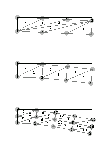
Compare the displacement graphically. The endpoint displacements approach the theoretical values as the mesh becomes more regular and refined.
In[226]:=Show[GraphicsArray[{{pl1},{pl2},{pl3}}]];
5.4.9 Mesh Generation: Isoparametric Formulation
Techniques Based on Rectangular Elements
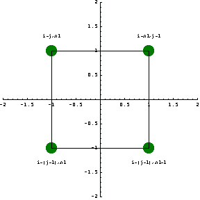
This section shows how you use a rectangular grid and isoparametric formulation to generate a mesh for simple two-dimensional shapes. It uses the following numbering schema for grid (nodal) points where i, j, and  denote the column number, the row number, and the number of grids in the x-direction in a row, respectively. denote the column number, the row number, and the number of grids in the x-direction in a row, respectively.
In[227]:=Show[
Graphics[{Text["i+(j-1)*n1",{-1.0,-1.3}],
Text["i+(j-1)*n1+1",{1.0,-1.3}],
Text["i+n1*j+1",{1.,1.3}],
Text["i+j*n1",{-1.,1.3}]}],
ElementPlot[{{{-1,-1},{1,-1},{1,1},{-1,1}}},
NodeColor->RGBColor[0,.5,0],
DisplayFunction->Identity],
PlotRange->{{-2,2},{-2,2}},
Axes->True,
AspectRatio->1];
Generate the nodal points of a square grid consisting of six grids in each direction.
In[228]:=n1=6;
n2=6;
nds=Table[{i+(j-1) n1,i + (j-1) n1 +1,i+1+j n1,i+j n1},
{i,1,n1-1},
{j,1,n2-1}];
The node numbers of the first element (for i = 1, 2; j = 1, 2; and  = 6). = 6).
In[232]:=nds[[1,1]]
Out[232]=
You need to convert nds, which is given in matrix form, into a list of four elements, and label the elements in a sequence. This will produce the connectivity matrix of the mesh.
In[233]:=pt=Partition[Flatten[nds],4];
In[234]:=con=(k=0;Map[{++k,#}&,pt]);
Now determine the coordinates of the grid points. First find the coordinate of the bottom-left point.
In[235]:=xo=-1;
yo=-1;
Next calculate the width and height of the square grid, and the corresponding element sizes.
In[237]:=xlength=2;
ylength=2;
dx=xlength/(n1-1);
dy=ylength/(n2-1);
Generate the coordinates of the previous nodal points pt.
In[241]:=pts=Partition[Flatten[Table[{xo+(i-1)dx,yo+(j-1)dy},
{j,1,n2},{i,1,n1}]],2];
This produces the mesh that is specified by the nodal points pts, the connectivity matrix con, and a number of MeshPlot options.
In[242]:=MeshPlot[pts,con,
PlotRange->1.2{{-1,1},{-1,1}},
AspectRatio->1,
Axes->True];
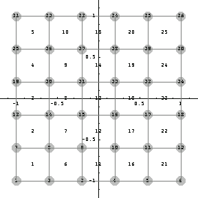
Now generate the interpolation functions that you can use in the isoparametric formulation and mapping of this grid. These are the coordinates of the master element that you adopt in this example.
In[243]:=xyco={{1,1},{1,-1},{1,0},{-1,1},{-1,-1},{-1,0},{0,1},{0,-1},{0,0}};
Give the locations of the nodal point in the element.
In[244]:=me=ElementPlot[{{{1,1},{1,-1},{-1,-1},{-1,1}},{1,0},{-1,0},{0,1},{0,-1},{0,0}} ,
AspectRatio->1,
PlotRange->{{-2,2},{-2,2}},
Axes->True];
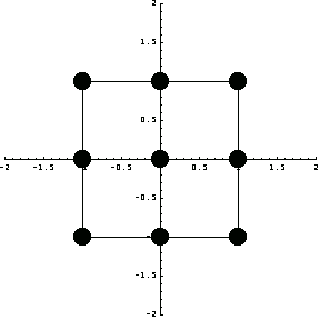
Then calculate the completeness information for this nine-node element and obtain the interpolation functions.
In[245]:=nodes9=RectangularCompleteness[9,0,0];
nodes9//TableForm
Out[246]//TableForm=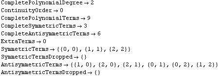
In[247]:=f9=ShapeFunctions2D[nodes9,xyco,{x,y}];
f9//TableForm
Out[248]//TableForm=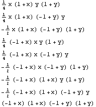
Here are the x and y coordinates of the isoparametric lines defined by the interpolation functions  and the nine interpolation points. and the nine interpolation points.
In[249]:=xco=f9.{x1,x2,x3,x4,x5,x6,x7,x8,x9};
yco=f9.{y1,y2,y3,y4,y5,y6,y7,y8,y9};
Isoparametric Curves on the Deformed Element
Use 25 isoparametric lines in the x- and y-directions. The variables lengthx and lengthy stand for the width and the height of the original element, and dx and dy denote the sampling intervals in the x- and y-directions.
In[251]:=nx=25;
ny=25;
lengthx=2.;
lengthy=2.;
dx=lengthx/nx;
dy=lengthy/ny;
As shown here, xnodes and ynodes are the x- and y- coordinates of the deformed element. The functions xmap and ymap are the mapping functions from the original element coordinates to the deformed element coordinates.
In[257]:=Clear[xnodes,ynodes,xmap,ymap,cpx,cpy,p1,p2];
xnodes={x1->1., x2->1., x3->1.,
x4->-1.,x5->1.4,x6->-1.,
x7->0., x8->0., x9->0.};
In[259]:=xmap[x_,y_]=xco/.xnodes;
In[260]:=ynodes={y1->1., y2->-1.,y3->0.,
y4->1., y5->1.1,y6->0.,
y7->1., y8->-1, y9->0.};
In[261]:=ymap[x_,y_]=yco/.ynodes;
In[262]:=cpx=Table[{xmap[dx(nx/2+1-i),y],ymap[dx(nx/2+1-i),y]},
{i,1,nx+1}];
In[263]:=p1=ParametricPlot[Evaluate[cpx],{y,-1,1},DisplayFunction->Identity];
In[264]:=cpy=Table[{xmap[x,dy(ny/2+1-i)],ymap[x,dy(ny/2+1-i)]},{i,1,ny+1}];
In[265]:=p2=ParametricPlot[Evaluate[cpy],{x,-1,1},DisplayFunction->Identity];
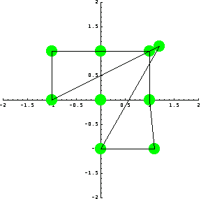
This example shows the coordinates of the deformed element, which are ordered such that the nodal points are connected in the correct sequence.
In[266]:=dpts={{{1.2,1.1},{0,-1},{1.1,-1.},{1.,0},{1.,1.},{0,1.},{-1,1.},{-1,0}},{0,0}};
In[267]:=de=ElementPlot[dpts,
AspectRatio->1,
DisplayFunction->$DisplayFunction,
PlotRange->{{-2,2},{-2,2}},
Axes->True,
NodeColor->RGBColor[0,1,0]];
In[268]:=
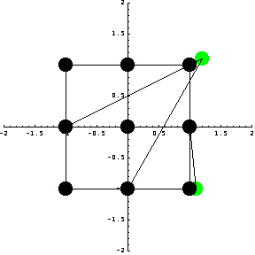
This produces the horizontal isoparametric lines on the original element.
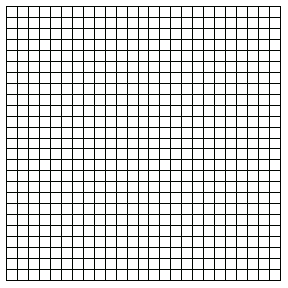
Next generate the vertical isoparametric lines on the original element.
In[269]:=cpx=Table[{dx(nx/2+1-i),y},{i,1,nx+1}];
In[270]:=p1=ParametricPlot[Evaluate[cpx],{y,-1,1},DisplayFunction->Identity];
In[271]:=cpy=Table[{x,dy(ny/2+1-i)},{i,1,ny+1}];
In[272]:=p2=ParametricPlot[Evaluate[cpy],{x,-1,1},DisplayFunction->Identity];
In[273]:=Show[p1,p2,
Axes->None,
AspectRatio->1,
DisplayFunction->$DisplayFunction];
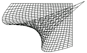
As earlier, you next generate the mapping of this 25 × 25 grid to the deformed coordinates.
In[274]:=Clear[xnodes,ynodes,xmap,ymap,cpx,cpy,p1,p2];
In[275]:=xnodes={x1->1, x2->1., x3->1.,
x4->-1,x5->1.4,x6->-1.,
x7->0, x8->0, x9->0.};
In[276]:=xmap[x_,y_]=xco/.xnodes ;
In[277]:=ynodes={y1->1, y2->-1.,y3->0,
y4->1.,y5->1.1,y6->0,
y7->1.,y8->-1, y9->0.};
In[278]:=ymap[x_,y_]=yco/.ynodes;
In[279]:=cpx=Table[{xmap[dx(nx/2+1-i),y],ymap[dx(nx/2+1-i),y]},{i,1,nx+1}];
In[280]:=p1=ParametricPlot[Evaluate[cpx],{y,-1,1},DisplayFunction->Identity];
In[281]:=cpy=Table[{xmap[x,dy(ny/2+1-i)],ymap[x,dy(ny/2+1-i)]},{i,1,ny+1}];
In[282]:=p2=ParametricPlot[Evaluate[cpy],{x,-1,1},DisplayFunction->Identity];
This generates the superimposition of the vertical and horizontal isoparametric lines in the deformed element.
In[283]:=Show[p1,p2,
Axes->None,
DisplayFunction->$DisplayFunction];
Waist
In this example, relocate the nodes of the master element and compute the mapping functions. The lists xnodes and ynodes denote the locations of the nodal points of the deformed mesh. The mapping functions in the x- and y-coordinates are xmap and ymap, respectively.
In[284]:=xnodes={x1->.8, x2->1.2, x3->.6,
x4->-.8,x5->-1.2,x6->-.6,
x7->0, x8->0, x9->0.};
In[285]:=xmap[x_,y_]=xco/.xnodes ;
In[286]:=ynodes={y1->1, y2->-1.1, y3->0,
y4->1., y5->-1.1, y6->0,
y7->1.1,y8->-.7, y9->0.};
In[287]:=ymap[x_,y_]=yco/.ynodes;
In[288]:=Transpose[{Map[#[[2]]&,xnodes],Map[#[[2]]&,ynodes]}]
Out[288]=
Order the nodes of the deformed element so that you can mark its boundary with the plotting function ElementPlot.
In[289]:=dpts={{{-1.2,-1.1},{0,-0.7},{1.2,-1.1},{0.6,0},{0.8,1.},{0,1.1},{-0.8,1.},{-0.6,0}},{0,0}};
This is how the boundary of the deformed element looks.
In[290]:=de=ElementPlot[dpts,
AspectRatio->1,
DisplayFunction->$DisplayFunction,
PlotRange->{{-2,2},{-2,2}},
Axes->True];
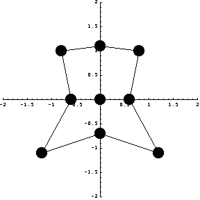
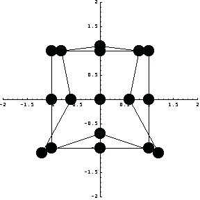
Visualize the magnitude of the displacements of the nodal points by superimposing de and me.
In[291]:=Show[de,me];
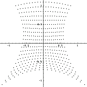
In order to study the effect of this mapping on the interior of the element, partition the original domain into 20 × 20 squares, and map the nodes of these squares to the deformed domain.
In[292]:=pl=Table[{xmap[.1(11-j),.1(11-i)],ymap[.1(11-j),.1(11-i)]},{i,1,21},{j,1,21}];
ListPlot[Partition[Flatten[pl],2],AspectRatio->1];
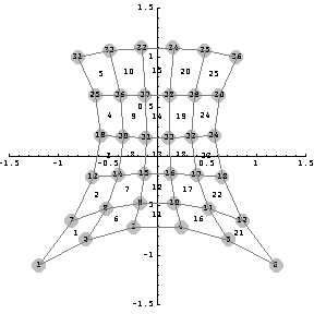
Similarly, you can map the nodal points of the mesh you generated earlier. You use the same connectivity matrix for both meshes so that the node numbers correspond to the same nodes in both meshes.
In[294]:=MeshPlot[Map[{xmap[##]&@@#,ymap[##]&@@#}&,pts],con,
PlotRange->1.5{{-1,1},{-1,1}},
AspectRatio->1,
Axes->True];
Simple Bridge
In this example, you will move some of the nodes of the master element a little further to generate a mesh for the bridge-like structure. The lists xnodes and ynodes denote the locations of the nodes in the deformed element. The functions xmap and ymap are the mapping functions.
In[295]:=xnodes={x1->5., x2->1., x3->3.,
x4->-5.,x5->-1.,x6->-3.,
x7->0, x8->0, x9->0.};
In[296]:=xmap[x_,y_]=xco/.xnodes ;
In[297]:=ynodes={y1->-1, y2->-1.,y3->-1,
y4->-1.,y5->-1.,y6->-1,
y7->1., y8->-.5,y9->0.};
In[298]:=ymap[x_,y_]=yco/.ynodes;
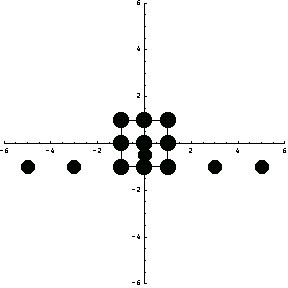
Unlike the previous mesh, the locations of the nodes are drastically changed as shown in this example.
In[299]:=dpts=Transpose[{Map[#[[2]]&,xnodes],Map[#[[2]]&,ynodes]}];
In[300]:=
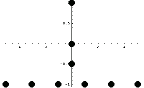
In[301]:=Show[me,de,PlotRange->{{-6,6},{-6,6}},AspectRatio->1];
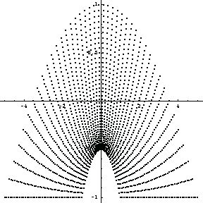
Now apply these maps to a mesh.
In[302]:=pnox=2 21;
pnoy=2 21;
dx=2/(pnox-1);
dy=2/(pnoy-1);
In[306]:=pl=Table[{xmap[dx((pnox-1)/2+1 1-j),dy((pnoy-1)/2+1-i)], ymap[dx((pnox-1)/2 +1 1-j),dy((pnoy-1)/2 + 1-i)]},{i,1,pnox},{j,1,pnoy}];
In[307]:=ListPlot[Partition[Flatten[pl],2],AspectRatio->1,PlotRange->All];
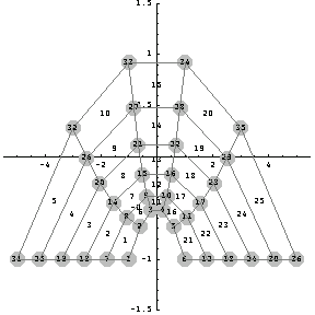
Here you plot the mesh for this model using the same procedure.
In[308]:=MeshPlot[Map[{xmap[##]&@@#,ymap[##]&@@#}&,pts],con,
PlotRange->{5.5{-1,1},1.5{-1,1}},
AspectRatio->1,
Axes->True];
Curved Beam
This section considers a curved beam and determines a mesh for it. Unlike the previous two examples, you will use elements in mappings, and a different type of master element.
In the following example, use the numbering schema for grid (nodal) points where i, j, and  denote the column number, the row number, and the number of grids in the x-direction in a row, respectively. denote the column number, the row number, and the number of grids in the x-direction in a row, respectively.
In[309]:=Show[Graphics[{ Text["i+(j-1)*n1" , {-1., -1.3}],
Text["i+(j-1)*n1+1", { 1., -1.3}],
Text["i+n1*j+1", { 1., 1.3}],
Text["i+j*n1", {-1., 1.3}]}],
ElementPlot[{{{-1,-1},{1,-1},{1,1},{-1,1},{-1,-1},{1,1}}},
DisplayFunction->Identity],
PlotRange->{{-2,2},{-2,2}},
Axes->True,
AspectRatio->1];
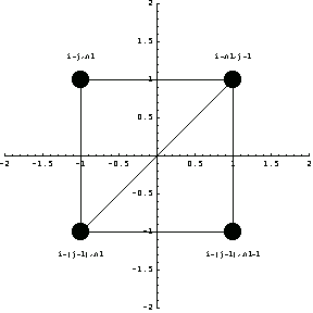
As before, you generate the connectivity matrix by using the numbering shown previously, and the coordinates of the nodal points.
In[310]:=n1=3;
n2=3;
In[312]:=nds=Table[{{i+(j-1) n1,i + (j-1) n1 +1,i+1+j n1},
{i+(j-1) n1,i+j n1,i+1+j n1} },
{i,1,n1-1},
{j,1,n2-1}];
In[313]:=pt=Partition[Flatten[nds],3];
In[314]:=con=(k=0;Map[{++k,#}&,pt]);
In[315]:=xo=0;
yo=0;
In[317]:=dx=10/(n1-1);
dy=2/(n2-1);
In[319]:=pts=Partition[Flatten[Table[{ xo+(i-1)dx, yo+(j-1)dy},
{j,1,n2},{i,1,n1}]],2];
In[320]:=f9beam=ShapeFunctions2D[nodes9,pts,{x,y}];
f9beam//TableForm
Out[321]//TableForm=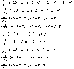
In[322]:=MeshPlot[pts,con,
PlotRange->{{-1,12},{-.5,2.5}},
AspectRatio->.4,
Axes->True];
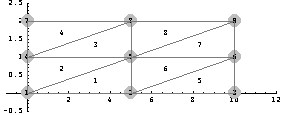
In[323]:=(k=0;Map[{++k,#}&,pts])
Out[323]=
Edit the last output in order to lift nodes 2, 5, and 8 in the y-direction by 0.5 unit length.
In[324]:=
Out[324]=
In[325]:=ptscurved=Map[#[[2]]&,%]
Out[325]=
MeshPlot produces the mesh corresponding to the coordinates of the curved beam. Notice that the connectivity of the mesh remains unchanged.
In[326]:=MeshPlot[ptscurved,con,
PlotRange->{{-1,12},{-.5,3}},
AspectRatio->.4,
Axes->True];
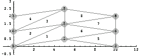
Here are the x and y components of the transformation.
In[327]:=Clear[xmap,ymap];
xmap[x_,y_]=f9beam.(Transpose[ptscurved][[1]]);
ymap[x_,y_]=f9beam.(Transpose[ptscurved][[2]]);
Now define a finer mesh for the same domain by specifying seven nodes in the x-direction and four nodes in the y-direction. Use the same procedure introduced previously.
In[330]:=n1=7;
n2=4;
In[332]:=nds=Table[{{i+(j-1) n1,i + (j-1) n1 +1,i+1+j n1},
{i+(j-1) n1,i+j n1,i+1+j n1}},
{i,1,n1-1},
{j,1,n2-1}];
In[333]:=pt=Partition[Flatten[nds],3];
In[334]:=con=(k=0;Map[{++k,#}&,pt]);
In[335]:=xo=0;
yo=0;
In[337]:=dx=10/(n1-1);
dy=2/(n2-1);
In[339]:=pts7=Partition[Flatten[Table[{ xo+(i-1)dx,yo+(j-1)dy},{j,1,n2},{i,1,n1}]],2];
Here is the undeformed mesh.
In[340]:=MeshPlot[pts7,con,
PlotRange->{{-1,12},{-.5,3}},
AspectRatio->.4,
Axes->True];
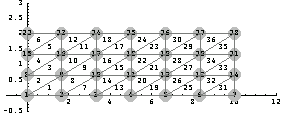
By mapping the nodal points to the curved element and keeping the same connectivity matrix, you can calculate the coordinates of the nodal points of the curved beam.
In[341]:=ptscurved=Map[{xmap[##]&@@#,ymap[##]&@@#}&,pts7];
Here is the mesh for the curved beam.
In[342]:=MeshPlot[ptscurved,con,
PlotRange->{{-1,12},{-.5,3}},
AspectRatio->.4,
Axes->True];
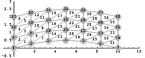
You may use the nodal points and the connectivity matrix for this mesh in a finite element analysis. You can further refine the mesh by changing the parameters  and and  . Also, you can simplify various other characteristics by the parameters introduced in this section, and many different configurations can be studied. . Also, you can simplify various other characteristics by the parameters introduced in this section, and many different configurations can be studied.
Techniques Based on Circular Elements
In addition to rectangular elements, you can use circular elements in generating meshes. Although they have certain limitations, circular elements can be quite effective in the meshes in which curves are dominant, such as arches and caps. This section explores the use of such elements in meshing circular domains and discusses the use of such elements.
Circular Elements
In a circular element, the interpolation functions correspond to nodal points in the radial direction for a constant radius. As a result, they are independent of the radius and are the only function of the radial coordinate. For example, here you can specify the nodal locations of five nodes.
In[343]:=pnodes={0, /2, /2, ,5 ,5 /4,7 /4,7 /4,2 /4,2 }; };
In[344]:=pon=Map[{#,1.}&,pnodes]
Out[344]=
In[345]:=poCarn=Map[{Cos[#[[1]]]#[[2]],Sin[#[[1]]]#[[2]]}&,pon];
Mark the locations of nodes by assuming that the radius of the element is unity.
In[346]:=mn=Show[ParametricPlot[{Cos[t],Sin[t]},{t,0,2 }, },
DisplayFunction->Identity],
ElementPlot[{poCarn},Axes->True,DisplayFunction->Identity],
AspectRatio->1,
PlotRange->{{-1.5,1.5},{-1.5,1.5}},
DisplayFunction->$DisplayFunction];
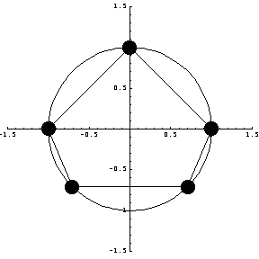
Use the function CircularElement to compute the shape functions for the element with these nodal points.


In[347]:=sf5=CircularElement[pnodes,x]
Out[347]=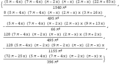
You can easily verify that each of these functions is zero everywhere except at their respective nodal points.
In[348]:=Map[(sf5/.x->#)&,pnodes]
Out[348]=
Mapping Parts
Here you use the transformation for the isoparametric representation.
In[349]:=pon={{0,1.},{ /2,.3},{ /2,.3},{ ,1.},{5 ,1.},{5 /4,1.},{7 /4,1.},{7 /4,1.},{2 /4,1.},{2 ,1.}}; ,1.}};
In[350]:=rho=N[sf5.Transpose[pon][[2]]];
theta=N[sf5.Transpose[pon][[1]]];
Deform the master element as follows.
In[352]:=poCarn=Map[{Cos[ #[[1]] ] #[[2]],Sin[ #[[1]] ] #[[2]]}&,pon];
In[353]:=p1=ElementPlot[{poCarn},
PlotRange->{{-1.5,1.5},{-1.5,1.5}},
Axes->True];
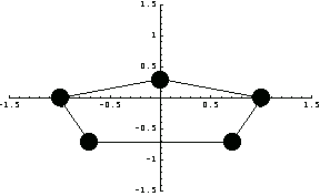
The next graph shows how you map the other points on the unit circle.
In[354]:=p2=Show[ParametricPlot[{Cos[t], Sin[t]},{t,0,2 },DisplayFunction->Identity],ParametricPlot[{rho Cos[theta],rho Sin[theta]}, },DisplayFunction->Identity],ParametricPlot[{rho Cos[theta],rho Sin[theta]},
{x,0,2 Pi},DisplayFunction->Identity],
PlotRange->All,
DisplayFunction->$DisplayFunction,
AspectRatio->1
];
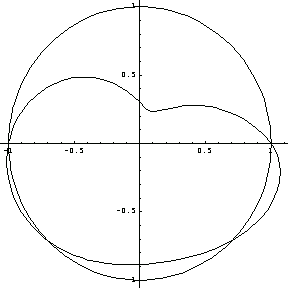
In[355]:=Show[p1,p2,AspectRatio->1];
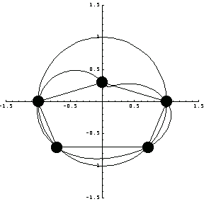
The lack of symmetry is attributed to the poor performance of the circular interpolation functions in general. This will become clear when these shape functions are plotted.
Two-Dimensional Circular Elements
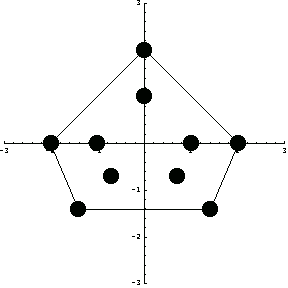
You calculate shape functions for an annulus domain by taking the cross product of those for a one-dimensional element and a circular element. In this example, the radii of the master elements are 1 unit and 2 units, respectively.
In[356]:=pon1=Map[{#,1.}&,pnodes];
pon2=Map[{#,2.}&,pnodes];
In[358]:=elp=ElementPlot[{Map[{Cos[ #[[1]] ] #[[2]],Sin[ #[[1]] ] #[[2]]}&,pon2],Map[{Cos[ #[[1]] ] #[[2]],Sin[ #[[1]] ] #[[2]]}&,pon1]},
PlotRange->{{-3,3},{-3,3}},
Axes->True,
AspectRatio->1];
In[359]:=Show[ParametricPlot[{Cos[t], Sin[t]},{t,0,2 },DisplayFunction->Identity], },DisplayFunction->Identity],
ParametricPlot[{2Cos[t], 2Sin[t]},{t,0,2 },DisplayFunction->Identity], },DisplayFunction->Identity],
elp,
DisplayFunction->$DisplayFunction,
PlotRange->2.5{{-1,1},{-1,1}},
AspectRatio->1];
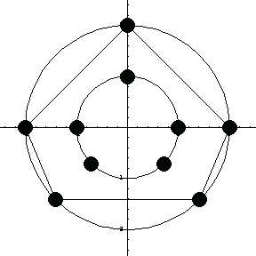
This calculates the shape functions for this concentric shape.
In[360]:=sf5=CircularElement[pnodes,tco];
sR=HermiteElement1D[{1,2},0,rco];
ce=Transpose[sR].{sf5};
Equivalently, you can use the function ConcentricElement2D.
In[363]:=ce2=ConcentricElement2D[{pnodes,{1,2}},{rco,tco}];


In[364]:=Map[ce/.{rco->2., tco-># }&, pnodes]//Chop
Out[364]=
In[365]:=Map[ce2/.{rco->2., tco-># }&, pnodes]//Chop
Out[365]=
Now rotate the outer circle of the annulus by  /10 and generate the mapping functions accordingly. /10 and generate the mapping functions accordingly.
In[366]:=n=6;
In[367]:=po1={{0,1.},{  /2,1.},{ /2,1.},{ ,1.},{5 ,1.},{5 /4,1.},{7 /4,1.},{7 /4,1.0},{2 /4,1.0},{2 ,1.}}; ,1.}};
In[368]:=po2={{0,2},{ /2,2. },{ /2,2. },{ ,2.},{5 ,2.},{5 /4,2.},{7 /4,2.},{7 /4,2.},{2 /4,2.},{2 ,2.}}; ,2.}};
In[369]:=po2=Map[{#[[1]]+Pi/10,#[[2]]}&,po2];
In[370]:=rho1=Sum[ce[[1]][[i]] po1[[i]][[2]],{i,1,n}]//N;
rho2=Sum[ce[[2]][[i]] po2[[i]][[2]],{i,1,n}]//N;
In[372]:=theta1=Sum[ce[[1]][[i]] po1[[i]][[1]],{i,1,n}]//N;
theta2=Sum[ce[[2]][[i]] po2[[i]][[1]],{i,1,n}]//N;
In[374]:=Clear[rho, theta, rco, tco];
In[375]:=rho[tco_,rco_]=rho1+rho2;
theta[tco_,rco_]=theta1+theta2;
In[377]:=ElementPlot[{Map[{Cos[#[[1]]]#[[2]],Sin[#[[1]]]#[[2]]}&,po2],Map[{Cos[#[[1]]]#[[2]],Sin[#[[1]]] #[[2]]}&,po1]},
PlotRange->All,
Axes->True];
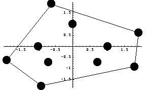
Original Mesh
In this example, you create a mesh for the annulus with 10 radial nodal points and 4 axial nodal points.
In[378]:=n1=10;
n2=4;
In[380]:=nds=Table[{i+(j-1) n1,i + (j-1) n1 +1,i+1+j n1,
i+j n1 },
{i,1,n1-1},
{j,1,n2-1}];
In[381]:=ins=Map[{#[[1]],#[[4]]}&,nds[[1]] ];
outs=Map[{#[[2]],#[[3]]}&,Last[nds] ];
gapc=
Table[
Flatten[{outs[[i]][[1]],ins[[i]],outs[[i]][[2]]}],
{i,1,Length[outs]}
];
In[384]:=conCir=Partition[Flatten[{nds,gapc}],4];
In[385]:=r1=1;
r2=3;
dtheta=2Pi/n1;
dr=(r2-r1)/(n2-1);
In[389]:=nodesRT=
Partition[
Flatten[
Table[{ (i-1)dtheta, r1+(j-1) dr},
{j,1,n2},
{i,1,n1}]
],
2]//N;
In[390]:=MeshPlot[Map[{#[[2]] Cos[#[[1]]],#[[2]] Sin[#[[1]]]}&,nodesRT],
(k=0;Map[{++k,#}&,conCir]),
PlotRange->All,
AspectRatio->1,
Axes->True];
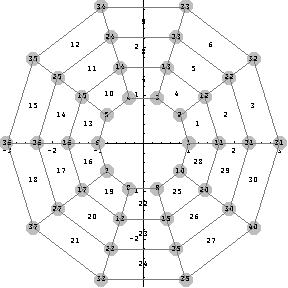
Mapped Mesh
Now apply the obtained mappings to the nodes of this rectangular mesh.
In[391]:=newRT=Map[{theta[##]&@@#,rho[##]&@@#}&,nodesRT];
nnds=Map[{#[[2]] Cos[#[[1]]],#[[2]] Sin[#[[1]]]}&,newRT];
ncon=(k=0;Map[{++k,#}&,conCir]);
In[394]:=MeshPlot[nnds,ncon,
PlotRange->All,
AspectRatio->1,
Axes->True];
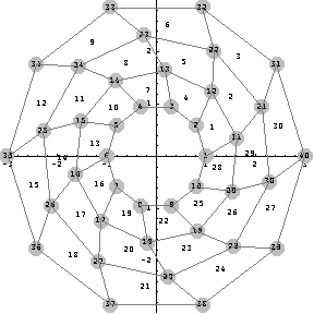
Triangular Elements
Repeat the same procedure with the triangular elements.
In[395]:=n1=10;
n2=4;
In[397]:=nds=Table[{{i+(j-1) n1,i + (j-1) n1 +1,i+1+j n1},
{i+(j-1) n1,i+j n1,i+1+j n1} },
{i,1,n1-1},
{j,1,n2-1}];
In[398]:=pt=Partition[Flatten[nds],3];
In[399]:=gaps=Table[{{(i-1)n1+1,i n1+1, (i+1)n1},
{(i-1)n1+1,i n1,(i+1)n1}},{i,1,n2-1}];
In[400]:=conCir=Partition[Flatten[{nds,gaps}],3];
In[401]:=r1=1;
r2=3;
dtheta=2Pi/n1;
dr=(r2-r1)/(n2-1);
In[405]:=nodesRT=
Partition[
Flatten[
Table[{ (i-1)dtheta, r1+(j-1) dr},
{j,1,n2},
{i,1,n1}]
],
2]//N;
In[406]:=pts=
Partition[
Flatten[
Table[{ xo + (i-1) dx, yo + (j-1) dy},
{j,1,n2},
{i,1,n1}]
],
2];
In[407]:=MeshPlot[Map[{#[[2]] Cos[#[[1]]],#[[2]] Sin[#[[1]]]}&,nodesRT],
(k=0;Map[{++k,#}&,conCir]),
PlotRange->All,
AspectRatio->1,
Axes->True];
|