2.2 Analysis of ARMA Time SeriesGiven a time series, we can analyze its properties. Since many algorithms for estimating model parameters assume the data form a zero-mean, stationary process, appropriate transformations of the data are often needed to make them zero-mean and stationary. The function ListDifference does appropriate differencing on ARIMA or SARIMA data. Note that all time series data should be input as a list of the form {x1, x2, ... } where xi is a number for a scalar time series and is itself a list, xi={xi1, xi2, ... , xim}, for an m-variate time series. | ListDifference[data, d] | difference data d times | | ListDifference[data, {d, D}, s] | difference data d times with period 1 and D times with period s |
Sample mean and transformations of data. After appropriate transformations of the time series data, we can calculate the properties of the series. The sample covariance function  for a zero-mean time series of n observations is defined to be  . The sample correlation function  is the sample covariance function of the corresponding standardized series, and the sample partial autocorrelation function is defined here as the last coefficient in a Levinson-Durbin estimate of AR coefficients. The sample power spectrum  is the Fourier transform of the sample covariance function  . The smoothed spectrum  using the spectral window {W(0), W(1), ... , W(M)} is defined to be  where W(k)=W(-k), while the smoothed spectrum  using the lag window { (0), (0),  (1), ... , (1), ... ,  (M)} (M)} is defined by  where  (k)= (k)= (-k) (-k). | CovarianceFunction[data, n]
CovarianceFunction[data1, data2, n] | give the sample covariance function of data or the cross-covariance function of data1 and data2 up to lag n | | CorrelationFunction[data, n]
CorrelationFunction[data1, data2, n] | give the sample correlation function of data or the cross-correlation function of data1 and data2 up to lag n | | PartialCorrelationFunction[data, n] | give the sample partial correlation function of data up to lag n | | Spectrum[data]
Spectrum[data1, data2] | give the sample power spectrum of data or the cross-spectrum of data1 and data2 | | SmoothedSpectrumS[spectrum, window] | give the smoothed spectrum using the spectral window window | SmoothedSpectrumL[cov, window,  ] ] | give the smoothed spectrum as a function of  using the lag window window |
Properties of observed data. The increasing magnitude of the data indicates a nonstationary series. We know this is the case, since it is generated from an ARIMA(1, 2, 0) process. Note that since the model has no MA part, the list of the MA parameters can be specified by { } or by {{0, 0 }, {0, 0 }}. | Out[2]= |  |
Differencing the above time series twice yields a new series that is stationary. | Out[3]= |  |
A SARIMA(2, 2, 0)(1, 1, 0) 2 series is transformed into a stationary series by differencing. | Out[4]= |  |
This generates a time series of length 200 from an AR(2) model. This computes the sample covariance function of the above series up to lag 5. | Out[6]= |  |
Here is the sample correlation function of the same series up to lag 5. Note that the correlation at lag 0 is 1. | Out[7]= |  |
This is the sample partial correlation function of the same series at lags 1 to 5. Note that the lag starts from 1 and not 0. | Out[8]= |  |
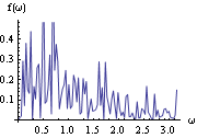
The power spectrum of the series is calculated here. This is the plot of the spectrum in the frequency range [0,  ]. | Out[10]= |  |
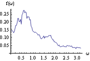
This gives the smoothed spectrum using the Daniell spectral window. We plot the smoothed spectrum. | Out[12]= |  |
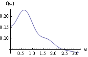
This yields the smoothed spectrum using the Hanning lag window. This is the plot of the smoothed spectrum. | Out[14]= |  |
We calculate the correlation function up to lag 2 from data generated from a vector MA(1) model. | Out[15]= |  |
When fitting a given set of data to a particular ARMA type of model, the orders have to be selected first. Usually the sample partial correlation or sample correlation function can give an indication of the order of an AR or an MA process. An AIC or a BIC criterion is also used to select a model. The AIC criterion chooses p and q to minimize the value of  by fitting the time series of length n to an ARMA( p, q) model (here  is the noise variance estimate, usually found via maximum likelihood estimation). The BIC criterion seeks to minimize  . | AIC[model, n] | give the AIC value of model fitted to data of length n | | BIC[model, n] | give the BIC value of model fitted to data of length n |
AIC and BIC values. Given a model, various methods exist to fit the appropriately transformed data to it and estimate the parameters. HannanRissanenEstimate uses the Hannan-Rissanen procedure to both select orders and perform parameter estimation. As in the long AR method, the data are first fitted to an AR( k) process, where k (less than some given kmax) is chosen by the AIC criterion. The orders p and q are selected among all p≤Min[pmax, k] and q≤"qmax" using BIC. | YuleWalkerEstimate[data, p] | give the Yule-Walker estimate of AR(p) model | | LevinsonDurbinEstimate[data, p] | give the Levinson-Durbin estimate of AR(i) model for i = 1, 2, ..., p | | BurgEstimate[data, p] | give the Burg estimate of AR(i) model for i = 1, 2, ..., p | | InnovationEstimate[data, q] | give the innovation estimate of MA(i) model for i = 1, 2, ..., q | | LongAREstimate[data, k, p, q] | give the estimate of ARMA(p, q) model by first finding the residuals from AR(k) process | | HannanRissanenEstimate[data, kmax, pmax, qmax] | give the estimate of the model with the lowest BIC value | | HannanRissanenEstimate[data, kmax, pmax, qmax, n] | give the estimate of the n models with the lowest BIC values |
Estimations of ARMA models. This generates a vector AR(2) series. Observe how the vector time series data are defined and input into functions below. | Out[17]//Short= |  |
The Yule-Walker estimate of the coefficients of the AR(2) series and the noise variance are returned inside the object ARModel. | Out[18]= |  |
Here the AR( p) ( p≤3) coefficients and noise variance are estimated using the Levinson-Durbin algorithm. Note that the small magnitude of  3 3 for AR(3) indicates that p=2 is the likely order of the process. | Out[19]= |  |
The same parameters are estimated using the Burg algorithm. | Out[20]= |  |
This gives the estimate of MA( q) ( q≤4) coefficients and noise variance using the innovations algorithm. | Out[21]= |  |
This estimates the same parameters using the long AR method. The data are first fitted to an AR(10) model. The residuals together with the data are fitted to an MA(2) process using regression. | Out[22]= |  |
Here the parameters of the ARMA(1,2) model are estimated using the long AR method. | Out[23]= |  |
This calculates the AIC value for the model estimated above. | Out[24]= |  |
The Hannan-Rissanen method can select the model orders as well as estimate the parameters. Often the order selection is only suggestive and it should be used in conjunction with other methods. | Out[25]= |  |
Here we select three models using the Hannan-Rissanen method. | Out[26]= |  |
This gives the BIC value for each model estimated above. | Out[27]= |  |
MLEstimate gives the maximum likelihood estimate of an ARMA type of model by maximizing the exact likelihood function that is calculated using the innovations algorithm. The built-in function FindMinimum is used and the same options apply. Two sets of initial values are needed for each parameter, and they are usually taken from the results of various estimation methods given above. Since finding the exact maximum likelihood estimate is generally slow, a conditional likelihood is often used. ConditionalMLEstimate gives an estimate of an ARMA model by maximizing the conditional likelihood using the Levenberg-Marquardt algorithm. | ConditionalMLEstimate[data, p] | fit an AR(p) model to data using the conditional maximum likelihood method | | ConditionalMLEstimate[data, model] | fit model to data using the conditional maximum likelihood method with initial values of parameters as the arguments of model | MLEstimate[data, model, { 1, { 1, { 11, 11,  12}}, ...] 12}}, ...] | fit model to data using maximum likelihood method with initial values of parameters {  1 1,  1 2}, ... | | LogLikelihood[data, model] | give the logarithm of Gaussian likelihood for the given data and model |
Maximum likelihood estimations and the logarithm of Gaussian likelihood. | option name | default value | | | MaxIterations | 30 | maximum number of iterations in searching for minimum |
Option for ConditionalMLEstimate. A vector AR(1) series of length 200 is generated. This yields the conditional maximum likelihood estimate of the parameters of a vector AR process. In the absence of an MA part, this estimate is equivalent to a least squares estimate and no initial values for parameters are needed. | Out[29]= |  |
This gives the conditional maximum likelihood estimate of an ARMA(2,1) model. The initial parameter values (  1=0.4, 1=0.4,  2=-0.35, 2=-0.35,  1=0.6 1=0.6) have to be provided as the arguments of ARMAModel. | Out[30]= |  |
The Hannan-Rissanen method is used to select a model. The estimated model parameters can serve as the initial values for parameters in maximum likelihood estimation. | Out[31]= |  |
The above result is input here for the conditional maximum likelihood estimate. | Out[32]= |  |
A SARIMA(1, 0, 1)(0, 0, 1) 2 series is generated. This yields the maximum likelihood estimate of the parameters of a SARIMA(1, 0, 1)(0, 0, 1) 2 model. Note that the parameters to be estimated are entered symbolically inside model and two initial values are needed for each of them. Since the calculation of the likelihood of a univariate series is independent of the noise variance, it should not be entered in symbolic form. | Out[34]= |  |
A bivariate MA(1) series is generated. For a vector ARMA series, the calculation of maximum likelihood is not independent of the covariance matrix; the covariance matrix has to be input as symbolic parameters. | Out[36]= |  |
This gives the logarithm of the Gaussian likelihood. | Out[37]= |  |
Let  =( =( 1, 1,  2, ... , 2, ... ,  p, p,  1, 1,  2, ... , 2, ... ,  q) q) be the parameters of a stationary and invertible ARMA( p, q) model and  the maximum likelihood estimator of  . Then, as n→ , we have  . For a univariate ARMA model, AsymptoticCovariance[model] calculates the asymptotic covariance V from model. The function InformationMatrix[data, model] gives the estimated asymptotic information matrix whose inverse can be used as the estimate for the asymptotic covariance. | AsymptoticCovariance[model] | give the covariance matrix V of the asymptotic distribution of the maximum likelihood estimators | | InformationMatrix[data, model] | give the estimated asymptotic information matrix |
Asymptotic covariance and information matrix. This gives the asymptotic covariance matrix of the estimators of an MA(3) model. The above asymptotic covariance is displayed in matrix form. | Out[39]//MatrixForm= |  |
This gives the estimate of the information matrix. The above information matrix is displayed here. | Out[41]//MatrixForm= |  |
There are various ways to check the adequacy of a chosen model. The residuals  of a fitted ARMA( p, q) process are defined by  where t=1, 2, ... , n. One can infer the adequacy of a model by looking at the behavior of the residuals. The portmanteau test uses the statistic  where  is the sample correlation function of the residuals; Qh is approximately chi-squared with h-p-q degrees of freedom. Qh for an m-variate time series is similarly defined, and is approximately chi-squared with m2(h-p-q) degrees of freedom. | Residual[data, model] | give the residuals of fitting model to data | | PortmanteauStatistic[residual, h] | calculate the portmanteau statistic Qh from residual |
Residuals and test statistic. The adequacy of the fitted model for the earlier example is accepted at level 0.05 for h=20 since  . | Out[42]= |  |
After establishing the adequacy of a model, we can proceed to forecast future values of the series. The best linear predictor is defined as the linear combination of observed data points that has the minimum mean-square distance from the true value. BestLinearPredictor gives the exact best linear predictions and their mean squared errors using the innovations algorithm. When the option Exact is set to False the approximate best linear predictor is calculated. For an ARIMA or SARIMA series {Xt} with a constant term, the prediction for future values of {Xt} can be obtained from the predicted values of {Yt}, { } }, where Yt=(1-B)d(1-Bs)DXt, using IntegratedPredictor. | BestLinearPredictor[data, model, n] | give the prediction of model for the next n values and their mean square errors | | IntegratedPredictor[xlist, {d, D}, s, yhatlist] | give the predicted values of {Xt} from the predicted values yhatlist |
Predicting time series. | option name | default value | | | Exact | True | whether to calculate exactly |
Option for BestLinearPredictor. This gives the prediction for the next three data points and their mean square errors for the vector ARMA(1, 1) process. | Out[43]= |  |
Here is the prediction for the next four data points and their mean square errors for the previously fitted SARIMA(1, 0, 1)(0, 0, 1) 2 model. | Out[44]= |  |
Here is the prediction for the next four data points and their mean square errors for an ARIMA(2, 2, 2) model. | Out[45]= |  |
|