|
2.3 The Kalman FilterThe Kalman filter is a technique that can be used to recursively estimate unobservable quantities called state variables, {Xt}, from an observed time series {Yt}. Many time series models (including the ARMA models) can be cast into a state-space form given by where {Yt} is the time series we observe and {Xt} is the state variable. F, G, c, and d are known matrices or vectors, and they can be dependent on time. {Wt} and {Vt} are independent Gaussian white noise variables with zero mean and covariance matrices  and  , respectively. Let  be the best linear estimate of Xt and Pt s s be its mean square error, given Is, the information up to time s. Given the initial values  , the Kalman filter yields  . KalmanFilter[Yt , { tt+1, Pt-1}, Ft+1, Gt, Qt+1, Rt, ct+1, dt] tt+1, Pt-1}, Ft+1, Gt, Qt+1, Rt, ct+1, dt] | give 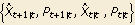 | KalmanFilter[{Ym+1, Ym+2, ..., YT}, { m+1|m, Pm+1|m}, F, G, Q, R, c, d] m+1|m, Pm+1|m}, F, G, Q, R, c, d] | give  , ...,  if F, G, R, c, and d are time independent |
Kalman filtering. Note that if any one of F, G, Q, R, c, ord is time dependent, F, G, Q, R, c, andd in the input to KalmanFilter shown above should be replaced by {Fm+2, Fm+3, ..., FT+1}, {Gm+1, Gm+2, ..., GT}, {Qm+2, Qm+3, ..., QT+1}, {Rm+1, Rm+2, ..., RT}, {cm+2, cm+3, ..., cT+1}, and {dm+1, dm+2, ..., dT}, respectively. Note also that if c 0 0 and d0, the last two arguments of KalmanFilter can be omitted. A fixed-point Kalman smoother gives the estimated value of the state variable at t based on all the available information up to T, where T>t. The idea is that as new data are made available, we can improve our estimation result from the Kalman filter by taking into account the additional information. | KalmanSmoothing[filterresult, F] | "smooth" the result of the Kalman filtering |
Kalman smoothing. KalmanSmoothing gives  . The first argument of KalmanSmoothing, filterresult, is the result of KalmanFilter, that is,
 , and F is the transition matrix in the above state equation. If F is time dependent, the second argument of KalmanSmoothing should be {Fm+2, Fm+3, ..., FT+1}. The Kalman prediction estimates the state variable Xt+h based on the information at t, It. KalmanPredictor[{ t+1|t, Pt+1|t}, F, Q, c, h] t+1|t, Pt+1|t}, F, Q, c, h] | give the next h predicted values and their mean square errors |
Kalman predictor. KalmanPredictor[ , F, Q, c, h] , F, Q, c, h] or KalmanPredictor[ ,{ ,{F t+2, ..., F t+h},{Q t+2, ..., Q t+h},{c t+2, ..., c t+h}] gives the next h predicted values and their mean square errors  . Again, the argument c can be omitted if it is always 0.
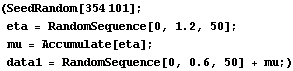
A simple structural model is the local level model. It is given by The model is in state-space form with F=1, G=1, and c=d=0. In the state-space model given earlier, if we set F=1, G=1, and c=d=0, we have a local level model. Here we generate a time series of length 30 according to the local level model with Q=1.2 and R=0.6. | Out[3]= | 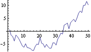 |
To start the Kalman filter iteration, initial values are needed. Here we use the so-called diffuse prior. | Out[4]= |  |
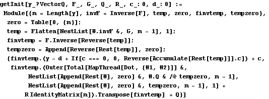
We can also use the function getInit to get the initial values. | Out[7]= |  |
This gives the result of Kalman filtering. Note that the initial values are  and the series now starts from t=2. Here the form of the output of KalmanFilter is shown. It is a list of  for t=2, 3, ..., T, with T=50. | Out[9]//Short= | 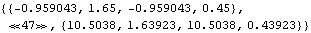 |
This gives the smoothed estimates of the trend and their mean square errors. Note that the output of KalmanSmoothing is a list of two lists. The first list contains  for t=2, 3, ..., T, with T=50 and the second list contains the corresponding mean square errors. | Out[11]= |  |
The smoothed values are plotted here. | Out[12]= | 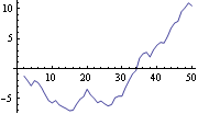 |
This gives the next three predicted values and their mean square errors. | Out[13]= |  |
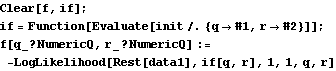
The Kalman filter can be used to calculate the likelihood function of a time series in state-space form. | LogLikelihood[data, init, F, G, Q, R, c, d] | give the logarithm of the Gaussian likelihood of data |
Log likelihood. Now the variances R and Q are to be estimated and the initial values depends on them. | Out[14]= |  |
This gives maximum likelihood estimate of Q and R. | Out[16]= |  |
|