1.1 IntroductionA discrete time series is a set of time-ordered data {xt1, xt2, ..., xtt, ..., xtn} obtained from observations of some phenomenon over time. Throughout this documentation we will assume, as is commonly done, that the observations are made at equally spaced time intervals. This assumption enables us to use the interval between two successive observations as the unit of time and, without any loss of generality, we will denote the time series by {x1, x2, ... xt, ... xn}. The subscript t can now be referred to as time, so xt is the observed value of the time series at time t. The total number of observations in a time series (here n) is called the length of the time series (or the length of the data). We will also assume that the observations result in real numbers, so that if at each time t a single quantity is observed, the resulting xt is a real number, and {x1, x2, ..., xn} is called a scalar or univariate time series. If at each time t several related quantities are observed, xt is a real vector and {x1, x2, ..., xn} corresponds to a vector or multivariate time series. The fundamental aim of time series analysis is to understand the underlying mechanism that generates the observed data and, in turn, to forecast future values of the series. Given the unknowns that affect the observed values in time series, it is natural to suppose that the generating mechanism is probabilistic and to model time series as stochastic processes. By this we mean that the observation xt is presumed to be a realized value of some random variable Xt; the time series {x1, x2, ... xt, ... }, a single realization of a stochastic process (i.e., a sequence of random variables) {X1, X2, ... Xt, ... }. In the following we will use the term time series to refer both to the observed data and to the stochastic process; however, X will denote a random variable and x a particular realization of X.
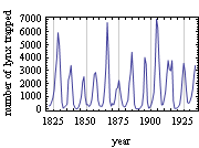
Examples of time series abound around us. Daily closing stock prices, monthly unemployment figures, the annual precipitation index, crime rates, and earthquake aftershock frequencies are all examples of time series we encounter. Virtually any quantity recorded over time yields a time series. To "visualize" a time series we plot our observations {xt} as a function of the time t. This is called a time plot. The following examples of time plots illustrate some typical types of time series. Example 1.1 The file lynx.dat in the directory TimeSeries/Data contains the annual number of lynx trapped in northwest Canada from 1821 to 1934. To plot the series we first need to read in the data; this is done by using ReadList. (See Section 1.4.1 for more on how to read in data from a file.) To plot the data we use the Mathematica function DateListPlot. Here is a plot of the lynx data. We see that there is a periodic oscillation with an approximate period of ten years. | Out[3]= |  |
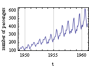
Example 1.2 The file airline.dat contains the data of monthly totals of international airline passengers in thousands from January 1949 to December 1960. It is read and plotted as a function of time. The airline passenger data is read in here. A plot of the airline passenger data shows a cyclic component on top of a rising trend. | Out[5]= |  |
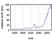
Example 1.3 Here is the time plot of common stock price from 1871 to 1970. The plot of the common stock price shows no apparent periodic structure with marked increase in later years. | Out[7]= |  |
The Time Series application package provides many of the basic tools used in the analysis of both univariate and multivariate time series. Several excellent textbooks exist that the reader may consult for detailed expositions and proofs. In this part of the manual we provide succinct summaries of the concepts and methods, introduce the functions that perform different tasks, and illustrate their usage. We first introduce some basic theoretical concepts and models used in time series analysis in Sections 1.2 and 1.3. Then in Section 1.4 we prepare data for modeling. Sections 1.5 and 1.6 deal with fitting a model to a given set of data, and Section 1.7 describes forecasting. Spectral analysis is the theme of Section 1.8. Section 1.9 introduces structural models and the Kalman filter. Section 1.10 deals with ARCH models and in the final section four data sets are analyzed using the methods introduced in this manual. |