1.5.1 Estimation of Covariance and Correlation FunctionsWe are given n observations {x1, x2, ... , xn} of a process {Xt} and we would like to estimate the mean and the covariance function of the process from the given data. Since, as we have mentioned before, the assumption of stationarity is crucial in any kind of statistical inference from a single realization of a process, we will assume in this section that the data have been rendered stationary using the transformations discussed in Section 1.4. We use the sample mean  as the estimator of the mean of a stationary time series {Xt}, and the sample covariance function  as the estimator of the covariance function of {Xt}, That is, the expectation in ( 2.8) is replaced by an average over the series at different times. It should be borne in mind that  and  defined in ( 5.1) and ( 5.2) are random variables, and for a particular realization of the time series {x1, x2, ... , xn} they give a particular estimate of the mean and the covariance function. Note that in the definition of the sample covariance, ( 5.2), the denominator is n although there can be fewer than n terms in the sum. There are other definitions of the sample covariance function that are slightly different from ( 5.2). For example, one definition uses n-k rather than n in the denominator. For the advantages of using ( 5.2), see the discussions in Kendall and Ord (1990), Sections 6.2 and 6.3 and in Brockwell and Davis (1987), p. 213. The sample correlation function  is defined to be the normalized sample covariance function, To calculate the sample mean from the given data we can use the function and to calculate the sample covariances and sample correlations up to lag k we can use the functions CovarianceFunction[data, k] and CorrelationFunction[data, k]. Note that these are the same functions we used to calculate theoretical covariance and correlation functions from a given model. The difference is in the first argument of these functions. To get the sample covariances or correlations from the given data, the first argument of these functions is the data instead of a model object. In principle, we can calculate the covariance or correlation up to the maximum lag n-1 where n is the length of the data. However, we should not expect  to be very reliable for k comparable to n since in this case there are too few terms contributing to the average in ( 5.2). However, if you want to calculate the correlation function up to the maximum lag often, you can define a function with the default lag value set to n-1 as follows. The lag argument is omitted from the function mycorrelation and it is assumed to be n-1. Example 5.1 Calculate the sample mean and sample correlation function from the data of length 500 generated from the AR(2) process Xt=0.9Xt-1-0.8Xt-2+Zt (see Example 2.6). We first generate the series according to the AR(2) model ARModel[{0.9, -0.8}, 1]. The random number generator is seeded first. This generates the time series of length 500 according to the given AR(2) model. Here is the sample mean of the series. | Out[5]= |  |
As we would have expected, the sample mean is close to the true mean 0. Next we calculate the sample correlation  up to lag k=25 and plot it against k. The plot of  versus the lag k is often referred to as the correlogram. This calculates the sample correlation function of the series up to lag 25. To plot the correlation function, we redefine the function plotcorr here. Here is the plot of the sample correlation function. We call this plot g2 for future re-display. | Out[8]= | 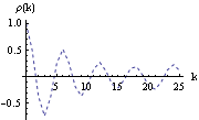 |
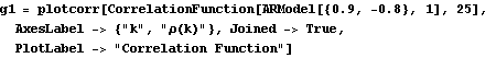
A dashed line is rendered due to the specification of the option PlotStyle. The number 0.02 inside Dashing specifies the length of the line segments measured as a fraction of the width of the plot. The theoretical correlation function calculated from the same model was displayed in Example 2.6. Here we display it again for comparison. This plots the theoretical correlation function of the AR(2) process. | Out[9]= | 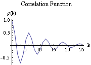 |
We can see how well the sample correlation function of the AR(2) process actually approximates the true correlation function by juxtaposing the plots of both using the command Show. The theoretical correlation function (solid line) and the sample correlation function (broken line) are displayed together here using Show. | Out[10]= |  |
We see that the sample correlation  provides a reasonable approximation to the true correlation function  (k) (k). Intuitively we also expect, by an application of the central limit theorem, that the larger the n, the better  approximates . This is indeed the case as we shall see in the next section. |