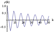
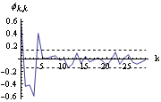
Legacy Documentation

There are various methods and criteria for selecting the orders of an ARMA model. We have seen in Sections 1.5.2 and 1.5.3 that the correlogram and partial correlogram can provide powerful tools to determine the order of a pure AR or MA process. So after the data have been transformed using the methods suggested in Section 1.4, the first thing to do is to look at the correlogram and partial correlogram. The failure of the sample correlation function to decay to zero sufficiently fast signals that further differencing may be necessary to make the data truly stationary.

Once the data are stationary, we can use our knowledge of theoretical correlation functions (see Section 1.2) of different models to deduce the possible ARMA orders for modeling our data. However, we must keep in mind that sample correlation functions do not always resemble the true correlation functions as well as in Example 5.1, especially in the small n case. Sample correlation at different lags can be highly correlated (see (5.4) for the expression of covariance of and ). Also it is easy to show that satisfies , even though the theoretical correlation function (k) is strictly positive for all k. (That is, is biased.)

Another type of order selection method is based on the so-called information criteria. The idea is to balance the risks of underfitting (selecting orders smaller than the true orders) and overfitting (selecting orders larger than the true orders). The order is chosen by minimizing a penalty function. The two commonly used functions are

and

Here is the estimated noise variance usually obtained from maximum likelihood estimations and n, as usual, is the length of the data. Akaike first suggested that the orders p and q be chosen such that they minimize the value of (5.8). This is called Akaike's information criterion (AIC). Similarly, using the minimum of (5.9) to select orders is called using Bayesian information criterion (BIC). (Other definitions of AIC use the logarithm of the likelihood function. See, for example, Brockwell and Davis (1987), p. 280.)

The first term in (5.8) and (5.9) can be interpreted as a penalty for underfitting, since the terms that are missing from the parameter fitting will be included in the noise and therefore give rise to an additional contribution to the noise variance. The second term in (5.8) and (5.9) is directly proportional to the number of ARMA parameters and it is clearly the penalty for overfitting. Its effect is to favor a parsimonious model. Choosing a model with the smallest possible number of parameters is an important principle in model selection, and this principle is referred to as the principle of parsimony. See Box and Jenkins (1970), Section 1.3.

To get the AIC or BIC value of an estimated model we can simply use

AIC[model, n] or BIC[model, n].

Since the calculation of these values requires estimated noise variance, we will postpone demonstrating the use of these functions until Section 1.6.

A seasonal ARIMA(p, 0, q)(P, 0, Q)_s model can, in principle, be treated as a special ARMA(p+sP, q+sQ) model in model selection. However, since the number of independent parameters involved is often much smaller than that of a general ARMA(p+sP, q+sQ) model, the principle of parsimony dictates that we should determine s, P, and Q as well as p and q. This usually presents additional difficulties in order selection. However, if the orders of the seasonal models are small, which often seems to be the case in practice, we can determine the seasonal period s by inspecting the correlogram using the theoretical properties of the correlation function we discussed in Section 1.3. The cutoff in the sample correlation or partial correlation function can suggest possible values of q+sQ or p+sP. From this we can select the orders of regular and seasonal parts.

First we look at the correlogram.

We see that the correlogram has extrema at lags that are multiples of 4. This suggests that s=4. Since the correlogram has no sharp cutoff, the model is unlikely to be a pure MA model. Next we look at the sample partial correlation function. We plot it along with the bounds .

The partial correlogram has a cutoff at lag k=5. We conclude that the model is a pure AR model with p+sP=5. Given that s=4, we may deduce that p=1 and P=1. This is, of course, an extremely simple example. In practice, model identification can be much more complicated.

For a mixed model we can select the orders using the AIC and BIC defined in (5.8) and (5.9) with p+q replaced by the number of seasonal model parameters p+P+q+Q.