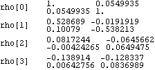
1.5.5 Order Selection for Multivariate Series For an m-variate series, Xt is a column vector of length m. The sample mean is again given by ( 5.1) and Mean[data] gives the estimate of the mean vector. The definition of sample covariance in the multivariate case is given by for 0≤k<n. The sample correlation function  is defined to be where  . Note that the above equation reduces to ( 5.3), the univariate sample correlation, when i=j. In fact, the correlation function is the covariance function of the normalized or standardized series (i.e., a series with zero mean and unit variance), which is obtained by subtracting from each component its mean and dividing by its standard deviation. Example 5.6 Calculate the sample correlation matrices up to lag 3 from the given bivariate data. The random number generator is seeded first. This generates a bivariate time series of length 80 from the given MA(1) model. The sample correlation function up to lag 3 is calculated and displayed in a table form. | Out[35]//TableForm= |  |
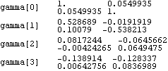
We can get the same result by calculating the sample covariance function  of the standardized data. The data can be standardized as follows. The series generated from the given MA(1) model is standardized. Each component of the standardized series data1 has mean zero. | Out[37]= |  |
The covariance function of the standardized data up to lag 3 is calculated and tabulated. | Out[38]//TableForm= |  |
This result is identical to the previous one. The variances of the series 1 and 2 are given by  ((0))11 ((0))11 and  ((0))22 ((0))22 and they are both 1. Also notice that  (k) (k) 0 0 for k>q=1. The methods of order selection employed in the univariate case can also be used for a multivariate series. The fact that an AR( p) process has vanishing partial correlations at lags greater than p and an MA( q) process has vanishing correlations at lags greater than q helps determine the order of an AR or MA process, respectively. For an MA( q) process, the asymptotic variance of the sample correlation  ( k>q) is given by for all i and j. If the cross-correlation between two series  ij(k) ij(k) vanishes for all k ( i.e., the two series are uncorrelated) and one of the series is a white noise process, the above formula for the variance of  reduces to This result can be used to test if two series are independent of each other. The sample partial correlation for a multivariate case is a direct extension of that for the univariate case. It is calculated using the Levinson-Durbin algorithm. Again, PartialCorrelationFunction[data, h] gives the sample partial correlation function up to lag h.
The AIC and BIC of an m-variate process use the penalty functions respectively. (  denotes the determinant of  .) They are again calculated using the functions AIC[model, n] and BIC[model, n] and can be used to select the orders of an m-variate ARMA process. |