Legacy Documentation

Sometimes there can be seasonal or cyclic components in a time series. By this we mean the recurrence of some recognizable pattern after some regular interval that we call the seasonal period and denote by s. For example, in the monthly data of international airline passengers there is clearly a recurring pattern with a seasonal period of 12.

A pure seasonal model is characterized by nonzero correlations only at lags that are multiples of the seasonal period s. This means that the time series at time t, X_t, depends on X_t-s, X_t-2s, X_t-3s, ... only. In general, we can define a pure seasonal ARMA model of orders P and Q and of seasonal period s by

If we define the seasonal AR polynomial (x^s) as

and the seasonal MA polynomial (x^s) as

(3.2) can be rendered more compactly using the backward shift operator B as

(Note that although we use the same notation and for seasonal model parameters as for multivariate ARMA model parameters, their meaning should be clear from the context.)

The pure seasonal models defined by (3.2) are often not very realistic since they are completely decoupled from each other. That is, (3.2) represents s identical but separate models for X_t, X_t+1, ... , X_t+s-1. In reality, of course, few time series are purely seasonal and we need to take into account the interactions or correlations between the time series values within each period. This can be done by combining the seasonal and regular effects into a single model. A multiplicative seasonal ARMA model of seasonal period s and of seasonal orders P and Q and regular orders p and q is defined by

Here (x) and (x) are regular AR and MA polynomials defined in (2.4) and (2.5).

To generalize the model defined by (3.3) to include nonstationary cases we define the seasonal difference to be (1-B^s)X_t=X_t-X_t-s. A multiplicative seasonal autoregressive integrated moving average (SARIMA) process of period s, with regular and seasonal AR orders p and P, regular and seasonal MA orders q and Q, and regular and seasonal differences d and D is defined by

We will use SARIMA(p, d, q)(P, D, Q)_s to refer to the model defined by (3.4). In typical applications, D=1 and P and Q are small.

A SARIMA(p, d, q)(P, D, Q)_s model is represented by the object

SARIMAModel[{d, D}, s, {₁, ... , _p}, {₁, ... , _p}, {₁, ... , _q},

{₁, ... , _Q},²].

Note that a pure seasonal model (3.2) and a seasonal ARMA model (3.3) are special cases of the SARIMA model, and we do not use different objects to represent them separately. If a particular order is zero, for example, p=0, the parameter list {₁, ... , _p} is {} or {0}. For example, ARMAModel[{},{}, 1] is the same as ARMAModel[{0},{},1] and as MAModel[{}, 1].

Any SARIMA process can be thought of as a particular case of a general ARMA process. This is because we can expand the polynomials on both sides of (3.4) and obtain an ARMA(p+Ps+d+sD, q+sQ) model whose ARMA coefficients satisfy certain relationships. Similarly, an ARIMA model defined in (3.1) is a special case of the ARMA(p+d, q) model. If we wish to expand a SARIMA or an ARIMA model as an equivalent ARMA model, we can invoke the function

ToARMAModel[model].

This is an ARMA(6, 4) model. In contrast to an arbitrary ARMA(6, 4) model, this model has only four independent ARMA parameters.

The functions introduced earlier for ARMA models are applicable to ARIMA and SARIMA models as well. These functions convert the ARIMA and SARIMA models to ARMA models internally and then compute the desired quantities. In the following we provide a few illustrative examples of the usage.

Since the covariance or correlation function is defined only for stationary models, any attempt to calculate the covariance or correlation function of a SARIMA or an ARIMA model with d≠0 or D≠0 will fail.

As expected, the covariance function of a pure seasonal model is nonzero only at lags that are multiples of the seasonal period s. The values of the covariance function at lags 0, s, 2s, ... are the same as those of a regular ARMA(P, Q) model with the same parameters. In fact, the two models are identical if we rescale time by a factor s in the pure seasonal model. In our current example, the values of the covariance function at lags 0, 3, 6, ... are the same as those at lags 0, 1, 2, ... of the regular ARMA(1, 1) model (1-₁B)X_t=(1+₁B)Z_t.

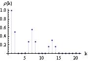
Since a SARIMA(p, 0, q)(P, 0, Q)_s model is an ARMA(p+sP, q+sQ) model, all the properties of the correlation and partial correlation functions we discussed in Sections 1.2.3 and 1.2.4 remain true. For example, the partial correlation function, _{k, k}, of a SARIMA(p, 0, 0)(P, 0, 0)_s model vanishes for k>p+sP, and the correlation function, (k), of a SARIMA(0, 0, q)(0, 0, Q)_s model vanishes for k>q+sQ. However, in some special cases we can say more about the correlation function of a seasonal ARMA model due to the relationships that exist between the coefficients. For example, the (q+sQ)^th degree polynomial (B)(B^s) can be expanded as

It is clear from the above expression that if s>q+1 there are "gaps" in the above polynomial, that is, terms from B^q+1 to B^s-1, from B^s+q+1 to B^2s-1, ... are absent. Now consider a seasonal ARMA model with p=P=0. The covariance function is given by

If these "gaps" are large enough, for some values of k the covariance function (k) vanishes simply because there is no overlap between the polynomials on the right-hand side of (3.5). In fact, if the "gap" (s-1)-(q+1)+1 is larger than q or s≥2(q+1), we have (k)=0 for q<k<s-q, s+q<k<2s-q, ... , (Q-1)s+q<k<Qs-q, and, of course, we always have (k)=0 for k>sQ+q.

It is also easy to show from (3.5) that as long as "gaps" exist (i.e., s>q+1) in the expansion of the MA polynomials, the covariance function is symmetric about the lags that are multiples of the seasonal period. In other words, (s-i)=(s+i), (2s-i)=(2s+i), ... for i=1, 2, ... , q.

Since p=P=0 and s=6≥2(q+1)=4, we expect the correlation function has the properties described above.

We observe that (a) (k)=0 for k>sQ+q=13; (b) (k)=0 for q=1<k<5=s-q and s+q=7<k<11=2s-q; and (c) (5)=(7), (11)=(13). We plot this correlation function.

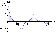
The symmetry of the correlation (k) about the lags that are multiples of the seasonal period s leads directly to the conclusion that at lags ks (k integer) the correlations are in general symmetric local extrema. This is seen clearly in the above graph.

The properties derived above for the correlation function of seasonal ARMA models with p=P=0 will not hold for general seasonal ARMA models. However, for some low-order seasonal models, which are often what we encounter in practice, the correlations at lags that are multiples of the seasonal period tend to be local extrema as shown in the following example. It is helpful to keep this in mind when identifying a seasonal model although fluctuations often wash out all but the very pronounced local extrema in practice. (See Section 1.5 on model identification.)

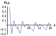
The calculation of the partial correlation function of a SARIMA model proceeds as in the case of an ARMA model. Again for q=Q=0, the partial correlation function _{k, k}=0 for k>p+sP.

Multivariate ARIMA and SARIMA models are again defined by (3.1) and (3.4), respectively, with (B), (B^s), (B), and (B^s) being matrix polynomials. All the functions illustrated above can be used for multivariate models; however, we will not demonstrate them here.