1.6.1 Parameter Estimation We first introduce some commonly used methods of estimating the parameters of the ARMA types of models. Each method has its own advantages and limitations. Apart from the theoretical properties of the estimators ( e.g., consistency, efficiency, etc.), practical issues like the speed of computation and the size of the data must also be taken into account in choosing an appropriate method for a given problem. Often, we may want to use one method in conjunction with others to obtain the best result. These estimation methods, in general, require that the data be stationary and zero-mean. Failure to satisfy these requirements may result in nonsensical results or a breakdown of the numerical computation. In the following discussion we give brief descriptions of each estimation method in the time series package; for more details the reader is urged to consult a standard time series text. Yule-Walker MethodThe Yule-Walker method can be used to estimate the parameters of an AR( p) model for a given p. If we multiply each side of ( 2.7) by Xt-k, k=0, 1, ... , p, and take expectations, we get a set of linear equations called the Yule-Walker equations: The Yule-Walker equations can be solved for the covariance function  given the AR parameters (in fact, the function CovarianceFunction for AR models is obtained by solving the Yule-Walker equations) or they can be solved for the AR coefficients { i} i} and the noise variance  2 2 if the covariance function is known. In practice, the exact covariance function is unknown and a natural way of getting an estimate of the AR parameters is to use the sample covariance function  to replace the corresponding theoretical covariance function  in ( 6.1) and ( 6.2) and solve for { i} i} and  2 2. The solution so obtained is called the Yule-Walker estimate of the AR parameters. In general, the method of estimating parameters by equating sample moments to theoretical moments is referred to as the method of moments. To estimate the parameters of an AR(p) model fitted to data using the Yule-Walker method we can use the function YuleWalkerEstimate[data, p]. It gives the estimated model object Example 6.1 Fit an AR(3) model to the data generated from the model Xt=0.9Xt-1-0.55Xt-2+0.4Xt-3+Zt using the Yule-Walker method. The random number generator is seeded first. A time series of length 120 is generated from the specified AR(3) model. Assuming that the order has been correctly identified we can proceed to estimate the parameters using the Yule-Walker method. This gives the estimated AR(3) model using the Yule-Walker method. | Out[4]= |  |
Note that the three numbers in the list are the estimated values of  1 1,  2 2, and  3 3, and the number 0.858176 is the estimated noise variance. Levinson-Durbin AlgorithmLevinson and Durbin derived an iterative way of solving the Yule-Walker equations. Instead of solving ( 6.1) and ( 6.2) directly, which involves inversion of a p p p matrix, the Levinson-Durbin algorithm fits AR models of successively increasing orders AR(1), AR(2), ... , AR( k) to the data. Let  and  be the jth AR coefficient and the noise variance of the fitted AR( m) model, respectively; the recursion formulas of the Levinson-Durbin algorithm are (see Brockwell and Davis (1987), Section 8.2 and Morettin (1984)) for k=1, 2, ... , m-1, and with  . The advantage of using the Levinson-Durbin algorithm over a direct solution of the Yule-Walker equations is that it also gives us the partial correlations { } }. (In fact, PartialCorrelationFunction uses the Levinson-Durbin algorithm to compute the partial correlation function.) This allows us to select an appropriate AR model in the process of the parameter estimation. The function LevinsonDurbinEstimate[data, k] fits models AR(1), AR(2), ... , AR(k) to data and gives a list of estimated model objects. Example 6.2 Use the Levinson-Durbin algorithm to fit an AR model to the data used in Example 6.1. This gives six estimated AR models of increasing order. | Out[5]= |  |
We can decide on the appropriate order by looking at the last AR( i) coefficient  i, i i, i for i=1, 2, ... , 6. This is precisely the sample partial correlation function defined earlier. To see this we can explicitly extract the last number in the list of AR coefficients of each model. The last AR coefficient of each model estimated above is extracted. | Out[6]= |  |
Whenever we want to extract an element from the same position in each entry in a list, we can use the All part specification. Here we wish to extract the last AR coefficient. The AR coefficients are the first parts of each ARModel and the last coefficient is the -1 part of that list. We get the same result using PartialCorrelationFunction. | Out[7]= |  |
We see that the partial correlations fall within the bound  (see ( 5.7)) for k>3. So we choose to model the data by an AR(3) process and the estimated model is the third entry in armodels. This extracts the third entry in armodels. | Out[8]= |  |
Note that this is exactly the same as the result we got in Example 6.1 by using YuleWalkerEstimate. We draw the attention of the reader to the behavior of the estimated noise variances. To see how they change as the order of the model is varied, we extract and plot them. The noise variances are extracted from armodels. | Out[9]= |  |
We plot the noise variance as a function of the AR model order p. | Out[10]= | 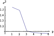 |
We see that initially the variance drops as we increase the order of AR model to be fitted, and after p=3 the variance levels off. This gives an indication that the true order of the model is probably p=3. This is because if the order of the fitted model is smaller than the true order, the noise variance will get an additional contribution from the terms that have been neglected and will be larger. Burg's AlgorithmBurg's algorithm (also referred to as the maximum entropy method) for estimating the AR parameters is also iterative, but it works directly with the data rather than with the sample covariance function. For large samples, Burg's algorithm is asymptotically equivalent to the Yule-Walker estimates although the two differ on small sample properties. For a presentation of Burg's algorithm see Jones (1978). The function fits AR(1), AR(2), ... , AR( k) models to data and gives a list of estimated model objects using Burg's algorithm. Example 6.3 Use Burg's algorithm to fit an AR model to the data from the AR(3) model studied in Example 6.1. This gives 5 estimated AR models using Burg's algorithm. | Out[11]= |  |
This is the estimated AR(3) model. Compare it with the result of the Levinson-Durbin algorithm in Example 6.2. | Out[12]= |  |
Innovations AlgorithmFor an MA model the method of moments involves solving a set of nonlinear equations and, therefore, it is not as convenient. Instead, other methods are used. The so-called innovations algorithm can be used to obtain a preliminary estimate of MA parameters. Fitting MA(1), MA(2), ... models to time series data using the innovations algorithm is analogous to fitting AR(1), AR(2), ... models to data using the Levinson-Durbin algorithm. The iterative formulas and the details of the derivation can be found in Brockwell and Davis (1987), pp. 165-166 and Section 8.3.
The function InnovationEstimate[data, k] allows us to use the innovations algorithm to get an estimate of the MA parameters. It gives the estimated models MA(1), MA(2), ... , MA( k). Let  be the jth MA coefficient of the estimated MA( m) model, then the asymptotic variance of  can be estimated to be and the order q is estimated to be the lag beyond which  lies within  for j>q. Once the order q is chosen, the estimated model parameters are given by  for j=1, 2, ... , q where m is sufficiently large that the values of  have stabilized with respect to m. In contrast, in the Levinson-Durbin algorithm, once the order of the AR process p is chosen, the estimated parameters for that p describe the estimated model. To illustrate how to get the estimate of an MA model, we generate a set of data from an MA(2) process and then try to fit an MA model to it. This seeds the random number generator. A time series of length 120 is generated from the given AR(2) model. Example 6.4 Fit an appropriate ARMA model to the given stationary time series data. We first look at the correlogram. This calculates the sample correlation function up to lag 25. To plot the correlation function, we redefine the function plotcorr here. The above sample correlation function corr is plotted using the function plotcorr. | Out[17]= | 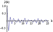 |
We see that  is small (<0.2) except for k≤2. We can conclude that the data are from an MA model of relatively small order. Next we calculate the bound for sample correlation function assuming q=1 (see ( 5.6)) The bound for the sample correlation function is calculated under the assumption that q=1. | Out[18]= |  |
The value of  is within the bound. | Out[19]= |  |
So MA(1) is a plausible model. Now we use the innovations algorithm to determine the MA order and estimate the parameters. This gives ten estimated MA models of increasing order using the innovations algorithm. | Out[20]= | 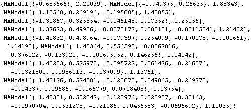 |
In order to compare the MA coefficients of the different models, let us extract and align them using the Mathematica function Column. The MA coefficients are extracted and aligned using Column. | Out[21]//NumberForm= |  |
We see that the MA coefficients  , j>2, lie within the bound  , suggesting that  j=0 j=0 for j>2. (Although one number  is larger than 0.18, it is within the bound  given by ( 6.3).) Since the MA coefficients  , j≤2, are significantly different from zero, we conclude that q=2. The values of  and  stabilize around -1.5 and 0.78, respectively. In fact, for m≥5 the fluctuations in  m, 1 m, 1 and  m, 2 m, 2 are of order  . So any  m, 1 m, 1 and  m, 2 m, 2 for m≥5 can be used as our estimated  1 1 and  2 2. We choose m=7 and find the estimated parameters by selecting the first two coefficients of the MA(7) model. This can be done conveniently using Mathematica. This extracts the MA(7) model and keeps only the first two MA coefficients. | Out[22]= |  |
Note that Map is used to perform an operation on all arguments while an operation on arguments only at specified locations is accomplished using MapAt. Long AR MethodFor a mixed model ARMA( p, q), the above methods are not applicable and we must resort to other techniques. The long AR method can be used to estimate the parameters of ARMA( p, q) models as well as AR( p) and MA( q) models. We may recall that an invertible ARMA model can be approximated by an AR( k) model for sufficiently large values of k. The long AR method of estimating ARMA parameters makes use of this fact. It first fits an AR( k) model ( k large, thus "long" AR method) to the data {xt}, The estimated AR( k) coefficients { } } are obtained using the ordinary least squares regression method. Then using the above equation with the { } } and data {xt}, we can get the estimated residuals or innovations { } }, Substituting these residuals into the ARMA( p, q) model we have, Now we can again use the ordinary least squares regression method to estimate the coefficients { i} i} and { i} i}, and the noise variance is given by the residual sum of squares divided by the number of terms in the sum, This procedure of fitting an invertible ARMA( p, q) model to data using the long AR method is encoded in the function LongAREstimate[data, k, p, q], where k is the order of long autoregression. Note that if the data are generated from a non-invertible model, long AR method fails and we may get nonsensical results. Example 6.5 Fit an MA(2) model to the data in Example 6.4 using the long AR method. The long AR method is used to obtain the estimated MA(2) model from data. | Out[23]= |  |
Example 6.6 Estimate the parameters of an ARMA(1, 2) model from the data generated below. The random number generator is seeded first. A time series of length 150 is generated from the given ARMA(1, 2) model. This gives the estimated ARMA(1, 2) model using the long AR method. The order of the long autoregression is 10. | Out[26]= |  |
Hannan-Rissanen ProcedureThe idea behind the Hannan-Rissanen procedure of estimating ARMA parameters is very similar to that behind the long AR method. That is, an AR( k) model is first fitted to the data in order to obtain the estimates of the noise or innovation zt; when this estimated noise  is used in place of the true noise it enables us to estimate ARMA( p, q) parameters using the less expensive method of least squares regression. However, the basic difference between the two methods is that in the long AR method the ARMA model orders to be fitted p and q as well as the order of long autoregression k, are supplied, whereas in the Hannan-Rissanen method the orders are determined within the procedure itself using an information criterion. Specifically, the Hannan-Rissanen procedure consists of following steps. 1. Use the Levinson-Durbin algorithm to fit models AR(i), for i=1, 2, ... , k"max", to the data.
2. Calculate the AIC values  for i=1, 2, ... , k"max" of the fitted AR models, and choose the model AR( k) that yields the smallest AIC value. 3. Calculate the residuals { } } from the fitted AR( k) model. 4. Estimate ARMA( p, q) coefficients using the least squares method for p≤"Min"(p"max", k) and q≤q"max"; the estimated noise variance is given again by ( 6.4). 5. Select the model that has the lowest BIC value (  ). For more details on the Hannan-Rissanen procedure see Granger and Newbold (1986), pp. 82-83. The function HannanRissanenEstimate[data, kmax, pmax, qmax] selects an appropriate ARMA model to fit the data using the Hannan-Rissanen procedure. Example 6.7 Use Hannan-Rissanen method to fit an ARMA model to the previous data. The Hannan-Rissanen procedure selects as well as estimates the model. It chooses an MA(1) model for the same data. | Out[27]= |  |
Instead of getting the model with the lowest BIC value as selected by the Hannan-Rissanen procedure, sometimes it is useful to know the models that have the next lowest BIC values. This can be done by specifying the optional argument in HannanRissanenEstimate. HannanRissanenEstimate[data, kmax, pmax, qmax, h] gives h estimated models with increasing BIC values. Computationally this does not cost any extra time. It is advisable to compare these h different models and decide on one in conjunction with other model identification methods. If you want to get all the models estimated in step 4 of the Hannan-Rissanen procedure, you can give a sufficiently large value of h. You can then select a model from these using your own criterion. Here we use the procedure to print out four models with the lowest BIC values. | Out[28]= |  |
To find the BIC and AIC values of these models we can use Map. We find the BIC values of each of the above four models. These values are in increasing order as they should be. | Out[29]= |  |
The AIC values of the models can be found similarly. | Out[30]= |  |
We see that while the MA(1) model has the lowest BIC value, the ARMA( 1, 2) model has the lowest AIC value. Next we plot the sample correlation. This calculates the sample correlation function up to lag 25. The above sample correlation function is plotted here. | Out[32]= | 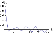 |
The bound for the sample correlation function is calculated under the assumption that q=1. | Out[33]= |  |
We see that although  is beyond this bound, there is no strong evidence to reject the MA(1) model. So based on the above analysis either MA(1) or ARMA(1, 2) can be tentatively identified as the right model. Maximum Likelihood MethodWhen the noise of a zero-mean, stationary ARMA process is normally distributed ( {Zt} N(0, N(0,  2) 2)), we can get the estimate of ARMA parameters by maximizing the Gaussian likelihood of the process. The parameters so obtained are called the maximum likelihood estimates of the parameters. The exact likelihood can be obtained from the prediction error decomposition (see Section 1.7) with the prediction errors being computed using the innovations algorithm. A complete discussion of the innovations algorithm and the calculation of the exact maximum likelihood can be found in Brockwell and Davis (1987), Chapter 5 and Sections 8.3 and 8.4. The function LogLikelihood[data, model] gives the logarithm of the exact Gaussian likelihood function for the given model and data. In the univariate case, LogLikelihood gives what is called the "reduced likelihood" (see Brockwell and Davis (1987), p. 250) and in the multivariate case, it gives the logarithm of the full maximum likelihood (apart from a constant). See Reinsel (1993), Section 5.4. Example 6.8 Calculate the logarithm of the likelihood of the estimated ARMA(1, 2) model in Example 6.7. Here is the logarithm of the likelihood of the ARMA( 1, 2) model estimated in Example 6.7. | Out[34]= |  |
The maximum likelihood method of estimating model parameters is often favored because it has the advantage among others that its estimators are more efficient ( i.e., have smaller variance) and many large-sample properties are known under rather general conditions. MLEstimate[data, model, { 1 , { 11, 11,  12}}, 12}}, ... ] fits model to data using the maximum likelihood method. The parameters to be estimated are given in symbolic form as the arguments to model, and two initial numerical values for each parameter are required. Internally the maximization of the exact logarithm of the likelihood is done using the Mathematica built-in function FindMinimum and the same options apply. (To find out all the options of FindMinimum use Options[FindMinimum].) Example 6.9 Use the maximum likelihood method to fit an MA(1) model and an ARMA(1, 2) model to the same data in Example 6.6. The maximum likelihood estimate of the MA(1) model is obtained using MLEstimate. | Out[35]= |  |
Similarly, this is the maximum likelihood estimate of the ARMA(1, 2) model. | Out[36]= |  |
This gives the logarithm of the likelihood of the latter model. | Out[37]= |  |
A couple of points of explanation are in order before we look at the results of our estimation. First, choosing good starting values for the parameters to be estimated is very important in the maximum likelihood estimation since not only can bad initial values slow down the calculation, but also abort the calculation if they reach the parameter region corresponding to nonstationary models. Since they are expected to be close to the values that maximize the likelihood, the estimated parameter values from other estimation methods are usually used as initial values for the maximum likelihood estimation as we have done here. This is why some authors call all the estimates of ARMA parameters that are not based on maximizing the likelihood function preliminary estimates, and use them primarily as initial values in maximizing the likelihood. Second, the alert reader may have noticed that the noise variance is not entered as a symbolic parameter. This is because in the univariate case, the likelihood function is independent of the noise variance and the noise variance is estimated separately at the end. So it does not matter what we input for the noise variance in the argument of the model, it is simply ignored. However, it is important that the noise variance should not be included in the parameter search list. This is because if extra parameters, which do not affect the value of the function being minimized, are included in the search list, FindMinimum will fail to find a minimum. Now we can select our model using AIC or BIC. The MA(1) model is favored by AIC. | Out[38]= |  |
The MA(1) model is also favored by BIC. | Out[39]= |  |
Both AIC and BIC favor the MA(1) model over the ARMA(1, 2) model. This result may be surprising, after all, we know that the data were generated from an ARMA( 1, 2) model. However, when n is small it is possible that other models can be fitted better to the data. More importantly, if the AR and MA polynomials  (x) (x) and  (x) (x) of an ARMA model have an approximate common factor of degree g, an ARMA( p-g, q-g) model rather than an ARMA( p, q) model is likely to be identified using information criteria. In our example, the MA polynomial  (x)=1+0.2x-0.5x2 (x)=1+0.2x-0.5x2 can be factorized as  (x)=(1-0.614143x)(1+0.814143x) (x)=(1-0.614143x)(1+0.814143x). The MA polynomial  (x)=1+0.2x-0.5x2 (x)=1+0.2x-0.5x2 contains a factor close to (1-0.6x). | Out[40]= |  |
We see that  (x)=(1-0.6x) (x)=(1-0.6x) and  (x) (x) share an approximate factor. This is why the data behave like an MA(1) model with  1 1 0.81 0.81. The large discrepancy between the estimated ARMA(1, 2) parameters and the "true" model parameters  1=0.6 1=0.6,  1=0.2 1=0.2, and  2=-0.5 2=-0.5 can also be explained by this accidental presence of an approximate common factor. Consider a series of data {xt} from an ARMA( p, q) model,  (B)xt= (B)xt= (B)zt (B)zt. It also satisfies an ARMA( p+g, q+g) model c(B) (B)xt=c(B) (B)xt=c(B) (B)zt (B)zt, where c(B) is a polynomial of degree g. If we fit an ARMA( p+g, q+g) model to the data, there is no unique solution and the maximum likelihood method can show strong dependence on the initial conditions. For example, if we change the initial conditions, we get quite different estimates from those in Out[36]. | Out[41]= |  |
Conditional Maximum Likelihood MethodIt is well known that the exact maximum likelihood estimate can be very time consuming especially when p+q is large. (We warn the user here that the function MLEstimate can be rather slow for large n or large number of parameters.) Therefore, often, when the data length n is reasonably large, an approximate likelihood function is used in order to speed up the calculation. The approximation is made by setting the initial q values of the noise zp, zp-1, ... , zp-q+1 to EZt=0 and fixing the first p values of X. The likelihood function so obtained is called the conditional likelihood function (conditional on zp=zp-1=... =zp-q+1=0 and on X1, X2, ... , Xp being fixed at x1, x2, ... , xp). Maximizing the conditional likelihood function is equivalent to minimizing the conditional sum of squares function. So the conditional maximum likelihood estimate is the same as the conditional nonlinear least squares estimate, and it is used as an approximation to the exact maximum likelihood estimate. Unlike the case of the least squares estimate, the conditional maximum likelihood estimate of the noise variance is given by the minimum value of the sum of squares divided by the effective number of observations n-p. The details of the conditional likelihood estimate are explained in Harvey (1981), Sections 5.2 and 5.3. See also Wilson (1973). The function ConditionalMLEstimate[data, model] can be used to fit model to data using the conditional maximum likelihood estimate. It numerically searches for the maximum of the conditional logarithm of the likelihood function using the Levenberg-Marquardt algorithm with initial values of the parameters to be estimated given as the arguments of model. Example 6.10 Fit a model to the data in Example 6.6 using the conditional maximum likelihood method. We use the result from the Hannan-Rissanen estimate as our initial values. We can input the output of the earlier calculation directly. The first model in hrmodels is used as the initial model to get the conditional maximum likelihood estimate of an MA(1) model. | Out[42]= |  |
The second model in hrmodels is used as the initial model to get the conditional maximum likelihood estimate of the ARMA( 1, 2) model. | Out[43]= |  |
For a pure AR model, the conditional maximum likelihood estimate reduces to a linear ordinary least squares estimate and no initial parameter values are necessary. We can if we like simply use ConditionalMLEstimate[data, p] to fit an AR( p) model to data. The Asymptotic Properties of the Maximum Likelihood EstimatorsOften we would like to know the approximate standard errors associated with our parameter estimates. These errors can be obtained from the asymptotic covariance of the estimators. Let  =( =( 1, 1,  2, ... , 2, ... ,  p, p,  1, 1,  2, ... , 2, ... ,  q) q) be the parameters of a stationary and invertible ARMA( p, q) model and  the maximum likelihood or conditional maximum likelihood estimator of  . Then, it can be shown that as n→ , To calculate V for a univariate ARMA model we can use the function AsymptoticCovariance[model]. The function uses the algorithm given in Godolphin and Unwin (1983). This gives the asymptotic covariance matrix V of the estimators of an MA(3) model. We display the covariance in matrix form. | Out[45]//MatrixForm= |  |
Similarly, the asymptotic covariance matrix V of the estimators of an ARMA( 1, 1) model is obtained but not displayed. This is the result after simplification. | Out[47]//MatrixForm= |  |
Although the function AsymptoticCovariance works for univariate ARMA models of arbitrary orders, the reader must be warned that with symbolic parameters the expressions can get very complicated with mixed models of even relatively small orders. However, with numerical parameters the covariance matrix is simply a (p+q) (p+q) (p+q) numerical matrix. In practice, the true parameter values are not known and the asymptotic covariance matrix is estimated by replacing the true model parameters with the estimated parameters. Another way of getting the approximate asymptotic covariance matrix is to calculate the approximate information matrix whose inverse is the desired covariance matrix. The approximation involves replacing the expectations with sample quantities. The function InformationMatrix[data, model] gives the estimated asymptotic information matrix from model and data. Example 6.11 Estimate the asymptotic covariance matrix of the estimated ARMA(1, 2) parameters in Example 6.10 using AsymptoticCovariance and inversion of InformationMatrix. This is the estimated asymptotic covariance V using the function AsymptoticCovariance. | Out[48]= |  |
We can also estimate V by inverting the information matrix. | Out[49]= |  |
The standard errors of  ,  , and  are given by the diagonal elements of  . This gives the standard errors of the estimated parameters. | Out[50]= |  |
Multivariate CaseAll of the above parameter estimation methods can be generalized to include multivariate models. The basic ideas are the same although the derivation and notation are considerably more involved. All the functions with the exception of AsymptoticCovariance given so far have been coded so that they can be used directly for multivariate cases. However, for maximum likelihood estimate there is one difference between the univariate and multivariate cases. In the multivariate case, the likelihood function is dependent on the covariance matrix, so the covariance matrix elements should be input as symbolic parameters and included in the parameter search list. The estimation of multivariate ARMA model can potentially involve large number of parameters even for small p and q. This can make the exact maximum likelihood estimation of the parameters computationally very slow. If in some cases one or more parameter values are known, then they should not be input as symbolic parameters, and they should not be included in the parameter search list. For example, in a bivariate AR(1) process, if for some reason ( 1)12 1)12 is fixed to be 0 then ARModel[{{{p1, 0}, {p3, p4}}}, {{s1, s2}, {s2, s4}}] should be input to the function MLEstimate reducing the number of parameters to six. Example 6.12 Fit a model to the given bivariate data using the Hannan-Rissanen method. The random number generator is seeded first. This generates a bivariate time series of length 200 from the given ARMA(1, 1) model. The Hannan-Rissanen procedure is used to select three models. | Out[53]= | 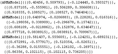 |
We obtain the orders of each of the three selected models. | Out[54]= |  |
We choose ARMA(1, 1) as our model, and use the conditional maximum likelihood method to further estimate the model parameters. We obtain the conditional maximum likelihood estimate of the selected model. | Out[55]= |  |
Next we calculate the standard errors of the estimated parameters. We first compute the asymptotic covariance matrix. The standard errors of { ,  ,  , ... ,  } } are given by the diagonal elements of  . The standard errors are obtained. | Out[57]= |  |
|