Legacy Documentation

In order to fit a time series model to data, we often need to first transform the data to render them "well-behaved". By this we mean that the transformed data can be modeled by a zero-mean, stationary ARMA type of process. We can usually decide if a particular time series is stationary by looking at its time plot. Intuitively, a time series "looks" stationary if the time plot of the series appears "similar" at different points along the time axis. Any nonconstant mean or variability should be removed before modeling. In this section we introduce a variety of methods of transforming the data.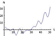

It is clear from the time plot that the series is not stationary since the graph shows a tendency to increase with t, signaling a possible nonconstant mean (t). A nonconstant mean (t) is often referred to as a trend. A trend of a time series can be thought of as an underlying deterministic component that changes relatively slowly with time; the time series itself can be viewed as fluctuations superimposed on top of this deterministic trend. Estimating the trend by removing the fluctuations is often called smoothing, whereas eliminating the trend in order to obtain a series with a constant mean is often called detrending.

There are various ways of estimating a trend. For example, we can assume that the trend can be approximated by a smooth function and use a simple curve-fitting method. The Mathematica function Fit can be used to fit a linear combination of functions to the data using linear least squares method. In this example, we fit a quadratic function of t (i.e., a linear combination of {1, t, t²}) to the above data. Fitting a polynomial in t to time series data using the least squares method is often referred to as polynomial regression.

This is the estimate of the trend. We can remove the trend and get the "detrended" data or residuals by subtracting the trend from the data.

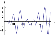This series now appears suitable for modeling as a stationary process.

In using the curve fitting method for estimating the trend described above we implicitly assumed that a global function fits the entire data. This is not always desirable and often methods of modeling the trend locally are preferable. For example, a simple moving average can be used to estimate the trend. Let y_t be the smoothed value (i.e., estimated trend) at t. A simple moving average of order r is defined by

Thus each new data point is the average of r previous data points. Short time fluctuations are averaged out leaving smoothed data, which we use as an estimate of the trend. The function

MovingAverage[data, r]

performs a simple moving average of order r on data and gives the smoothed data {y_t}.

Instead of using identical weights in the above sum, we can generalize the simple moving average by allowing arbitrary weights {c₀, c₁, ... , c_r}. This leads to a weighted moving average or linear filter. (An analysis of linear filters in the frequency domain will be found in Section 1.8.2.) Application of a linear filter of weights {c₀, c₁, ... , c_r} to {x_t} produces the filtered series {y_t} given by

This is sometimes referred to as a one-sided or causal filter and y_t=c_ix_t-i as a two-sided filter. The filter defined above is no less general than a two-sided one since a simple "time shifting" converts one kind of filter to the other.

The function

applies a moving average with weights {c₀, c₁, ... , c_r} to data. The weights are rescaled to sum to 1. For a more detailed discussion of moving averages see Kendall and Ord (1990), pp. 28-34.

Another kind of moving average is the so-called exponentially weighted moving average or exponential smoothing. In exponential smoothing, the weights decrease exponentially and the smoothed series is given by

where a is called the smoothing constant and is usually restricted to values between 0 and 1. An initial value of y₀ is required to start the updating. The function

ExponentialMovingAverage[data, a]

performs exponential smoothing on data with smoothing constant a. The initial value is taken to be the first element in data. A different starting value y₀ can be used by prepending y₀ to data.

An ARIMA(0, 1, 0) model is also called a random walk model. Here is the plot of 100 data points generated from a random walk model.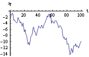

Again the graph shows that the data display a tendency to increase with t. We might infer that the process has a nonconstant mean (t). However, we know that the ARIMA model defined in Section 1.3 has mean zero, so this appearance of a nonstationary mean is the result of a single finite realization of a zero-mean nonstationary process. This apparent trend is often termed a stochastic trend in contradistinction to the deterministic trend we introduced earlier.

Differencing is an effective way of eliminating this type of trend and rendering the series stationary. Recall that the once-differenced data {y_t} is given by y_t=x_t-x_t-1=(1-B)x_t, and twice-differenced data by (1-B)y_t=x_t-2x_t-1+x_t-2=(1-B)²x_t. So the ARIMA(0, 1, 0) series after differencing is a stationary series (1-B)x_t=y_t=z_t. Similarly, an ARIMA(p, d, q) series can be transformed into a stationary series by differencing the data d times. To difference the data d times and get (1-B)^dx_t we can use

ListDifference[data, d].

Notice that differencing is really a particular kind of linear filtering and a polynomial trend of degree k can be eliminated by differencing the data k+1 times.

Now we difference the above random walk data and plot the differenced series.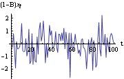

So far we have dealt with eliminating a nonconstant mean present in the time series. Nonstationarity can also be due to nonconstant variance. For example, in the plot of the airline data (Example 1.2) we see clearly an increase in the variance as t increases. Here we re-display its time plot for examination.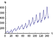

We see that the variance, riding on the trend, is also changing with time. We need to transform the series into a constant variance before modeling it further. To stabilize the variance, a nonlinear transformation such as a logarithmic or square-root transformation is often performed. In this example, we try a natural logarithmic transformation, y_t=lnx_t.

Th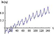e variance now is stabilized. However, the trend is still present and there is the obvious seasonality of period 12. The method of differencing can also be used to eliminate the seasonal effects. We define the seasonal difference with period s as x_t-x_t-s=(1-B^s)x_t.

We can difference the data d times with period 1 and D times with the seasonal period s and obtain (1-B)^d(1-B^s)^Dx_t using

ListDifference[data, {d, D}, s].

Here is the airline data after the logarithmic transformation and seasonal differencing with period 12.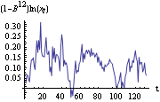

We see that the periodic behavior or seasonal effect has been eliminated. The series after removal of the seasonal component is often referred to as seasonally adjusted series or "deseasonalized" series. A further difference gives the following plot.

Th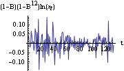is series (1-B)(1-B¹²)ln(x_t) can be fitted to a stationary model.

In fact, the logarithmic transformation is a special case of a class of transformations called the Box-Cox transformation. If we denote the transformed series by {y_t} and let be a real constant, the Box-Cox transformation is defined by

and

Different values of yield different transformations. It is trivial to implement this transformation on Mathematica. If data contains the time series data to be transformed then

(data-1)/

or

Log[data]

gives the transformed series.

Sometimes the nonstationarity can come from models not included in the ARIMA or SARIMA models. For example, the AR polynomial might have unit roots that are not 1. Since the AR coefficients are real, the complex roots on the unit circle will appear in complex conjugate pairs resulting in factors such as (1-eⁱB)(1-e^-iB)=(1-2cosB+B²) in our AR polynomial. We can use ListCorrelate[{1, -2 Cos[], 1}, data] to remove this kind of nonstationarity.

After the data have been rendered stationary, we are ready to fit an appropriate model to the data. This is the subject of the next two sections.