Legacy Documentation

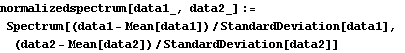
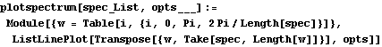
The spectrum of a time series can be obtained from previously stated formulation as long as we know the model satisfied by the time series. Often in practice we only have a finite set of time series data and we would like to estimate from it the spectrum of the process.

There are two commonly used approaches to estimating the spectrum. The first is called the ARMA method of spectrum estimation. In this way of estimating the spectrum, we first fit an appropriate ARMA type of model to the data and then get the estimated spectrum by replacing the true model parameters in (8.4) with the estimated ARMA parameters. The function Spectrum[model, w] gives the estimated spectrum as a function of with model here being the estimated model from the given data set.

Another approach to estimating spectrum is nonparametric, that is, it uses the time series data directly and no model is assumed a priori. A "natural" way of getting the estimate of f(), , is to replace the covariance function (k) in (8.1) by the sample covariance function ,

Here takes on continuous values in the range [-, ], and we call the continuous sample spectrum. Note that the sum in (8.5) is restricted to k<n, since for a time series of length n the sample covariance function can be calculated up to at most a lag of n-1. It is straightforward to write a one-line program that gives the continuous sample spectrum given the sample covariance function cov = and the frequency variable . For example, write (8.5) as . The continuous sample spectrum can be obtained using

cov[[1]]/(2Pi) + Rest[cov].Table[Cos[k ], {k, 1, Length[cov]-1}]/Pi.

In practice, it is often convenient to only consider defined on a set of discrete Fourier frequencies _j=2j/n for j=0, 1, ... , n-1. Let =_j in (8.5) and we call for j=0, 1, ... , n-1 the discrete sample spectrum. It turns out that computationally it is very convenient to calculate the discrete sample spectrum, since using the definition of the sample covariance function, (8.5) can be written at =_j as

where 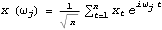is the discrete Fourier transform of x_t.

So the discrete sample spectrum is simply proportional to the squared modulus of the Fourier transform of the data. In the rest of the discussion we will drop the adjective "discrete" and use sample spectrum to mean . Periodogram is another name for essentially the same quantity. To get the sample spectrum of a given data {x₁, x₂, ... , x_n} use

Spectrum[data].

It gives for j=0, 1, ... , n-1. Internally, it simply uses the function Fourier. Although the definition of the Fourier transform here differs from that of Fourier by a phase factor, this phase factor will not enter in (8.6) due to the squared modulus. You can also define a function to estimate the normalized spectrum defined by (8.5) with in place of as follows.

If we just want to get some idea of what the sample spectrum looks like, we can simply do ListLinePlot[spec]. However, as we have mentioned before, ListLinePlot[spec] plots the sample spectrum {} against =1, 2, ... , n not =_j for j=0, 1, ... , n-1. A careful plot of the sample spectrum should use ListLinePlot to plot points . To avoid repeated typing we can define a function plotspectrum to plot sample spectrum.

Note that we only need the spectrum in the range [0, ] and the spectrum in (, 2) has been dropped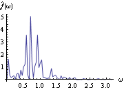.