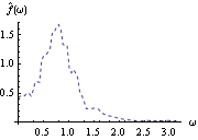
In general, the sample spectrum can fluctuate a lot and its variance can be large, as can be seen in the last example. In fact, the variance of the sample spectrum does not go to zero as the length of the time series n→. In other words, is not a consistent estimator of f(). In order to reduce the fluctuations in the sample spectrum, we often "smooth" the sample spectrum using weighted averages. There are two commonly used approaches to spectrum smoothing; they correspond to performing a weighted average in the frequency domain and in the time domain, respectively. In the following, we will show how to smooth a spectrum using both of the approaches and discuss the relationship between the two methods.

Let {W_n(k)} (k=-M, -(M-1), ... , (M-1), M) be a set of weights satisfying

In the following we will omit the subscript n in W_n(k), i.e., the n dependence of the weights is understood. Given a discrete sample spectrum we define its smoothed spectrum by

That is, the smoothed spectrum at frequency w_j=2j/n is the weighted average of the spectrum in the neighborhood [_j-M, _j+M] of _j. Since only frequencies in this range are "seen" in the averaging process, the set of weights {W(k)} is referred to as a spectral window. (The subscript S in stands for spectral window.) The function

SmoothedSpectrumS[spectrum, window]

smooths the given sample spectrum using the supplied spectral window. This function is very much like a weighted moving average since is obtained by an application of the filter {W(k)} on the sample spectrum. However, it differs in two respects: (a) the periodic nature of the sample spectrum (i.e., ) is taken into account in implementing (8.7), so the output of SmoothedSpectrumS (smoothed spectrum using spectral window) has the same length as the input spectrum; and (b) since W(k)=W(-k), we only need to input the spectral window as {W(0), W(1), ... , W(M)}.

Designing a window includes choosing an M and the appropriate weights. See Priestley (1981), Section 7.5 for details on how to choose a window. An often used spectral window is the Daniell window defined by W(k)=1/(2M+1) for k≤M and 0 otherwise (i.e., it is a rectangular window). Using the Daniell window to smooth the sample spectrum is the same as doing a simple moving average.

When M=6 the Daniell window is W(k)=1/(2M+1)=1/13. We can generate the list of M+1=7 identical weights using Table[1/13, {7}].

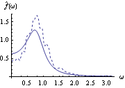
This spectrum closely resembles the theoretical spectrum calculated earlier for the same model (see g1 in Example 8.4). We display them together to see the resemblance using Show.

Changing windows or using different M for the Daniell window can greatly affect the shape of the smoothed spectrum. The reader is encouraged to try different windows and see their effect on smoothing.

Another approach to smoothing a spectrum is to perform averaging in the time domain. Instead of averaging the sample spectrum, we assign weights to the sample covariance function in (8.5) such that the contributions from covariance at large lags, which are generally not reliable, will be small or zero. Let {(k)} (k=-M, -(M-1), ... , M-1, M) be a set of weights satisfying

then {(k)} constitutes a lag window and M is called the truncation point. A smoothed spectrum using a lag window is defined by

The subscript L stands for lag window. Note that (8.8) has defined a continuous spectrum for =[-, ], not just for discrete Fourier frequencies. This is not too bad from a computational point of view since the truncation point M is generally small compared to n.

The function

SmoothedSpectrumL[cov, window, ]

gives the smoothed spectrum defined in (8.8). The argument cov is the sample covariance function calculated from the given time series data; the lag window specified by window is {(0), (1), ... , (M)}; and w is the frequency variable. Note that the truncation point M should not be greater than the largest lag in the covariance function cov. The advantage of using covariance function rather than the time series data directly as the input to SmoothedSpectrumL is that it allows us to try different windows or truncation points without having to recalculate the covariance function each time. Observe also the correspondence of the arguments in SmoothedSpectrumS, where the sample spectrum is weighted, and in SmoothedSpectrumL, where the sample covariance function is weighted.

We now list some commonly used lag windows.

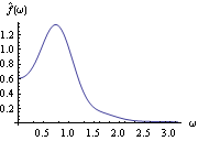
1. Rectangular or Truncated window: (k)=1 for k≤M, and (k)=0 for k>M.

2. Bartlett window: (k)=1-k/M for k≤M and 0 otherwise.

3. Blackman-Tukey window: (k)=1-2a+2acos(k/M) for k≤M and 0 otherwise. Here a is a constant in the range (0, 0.25]. When a=0.23, the window is called a Hamming window, and when a=0.25, a Hanning window.

4. Parzen window: (k)=1-6(k/M)²+6(k/M)³ for k≤M/2, (k)=2(1-k/M)³ for M/2<k≤M, and 0 otherwise.

It closely resembles the theoretical spectrum we plotted earlier (see g1 in Example 8.4). Again, different windows or truncation points can give different smoothed spectra.

While they appear to be quite different, the two approaches to smoothing spectrum are actually intimately related. If we define a spectral window with a continuous weight function W() as the Fourier transform of the lag window {(k)},

then

It is easy to show that

where is the continuous sample spectrum defined in (8.5), , and _j=2j/n. (See, for example, Brockwell and Davis (1987), pp. 348-349.) So smoothing in the time domain using the lag window {(k)} is the same as smoothing in the frequency domain using the spectral window W() and vice versa where W() and {(k)} are related through (8.9) and (8.10). At the Fourier frequencies the right-hand side of (8.11) is precisely defined in (8.7). Depending on the window, it may be easier to do the smoothing in one domain than in the other. For example, a lag window with small M (narrow width) translates into a spectral window with no cutoff and vice versa. Here we give a couple of spectral windows that correspond to the lag windows listed earlier.

The corresponding spectral window, or kernel, is obtained by evaluating the summation in (8.9).

This spectral window denoted by D_M() is often called the Dirichlet kernel of order M. We define it to be Di[M, ].

Whenever we want to use the Dirichlet kernel we can simply use Di[M, ]. Note that if is an integer multiple of 2 the limit with respect to can be used.

This is often referred to as Fejér kernel of order M, written as F_M(), and we define it to be F[M, ]. As with the Dirichlet kernel, the limit with respect to can be used for integer multiples of 2.

Similarly we can get the spectral window corresponding to Blackman-Tukey window. The result is a linear combination of Dirichlet kernels:

For the Parzen window, we need to evaluate the sum separately for M even and for M odd. When M is odd, use M-1 in place of M (M even) then substitute M back once the summation is done.

To demonstrate the equivalence of the two approaches we generate a time series of length 50 and calculate the smoothed spectrum using the Bartlett window (M=5) in both the time and frequency domains.

We first smooth the spectrum in the frequency domain using Fejér kernel. The weights {W(j)=W(_j)*2/n=F[5, 2j/50]*2/50} are generated using Table. F[5, 0]=5/(2) is added separately using Prepend to avoid taking the =0 limit.

At the frequencies _j=2j/50, j=0, 1, ... , 49, the difference between the two results should be small.