Legacy Documentation

In Example 2.1 we calculated the correlation function of an AR(1) process. Although X_t depends only on X_t-1, the correlations at large lags are, nevertheless, nonzero. This should not be surprising because X_t-1 depends on X_t-2, and in turn X_t-2 on X_t-3, and so on, leading to an indirect dependence of X_t on X_t-k. This can also be understood by inverting the AR polynomial and writing

Multiplying both sides of the above equation by X_t-k and taking expectations, we see that the right-hand side is not strictly zero no matter how large k is. In other words, X_t and X_t-k are correlated for all k. This is true for all AR(p) and ARMA(p, q) processes with p≠0, and we say that the correlation of an AR or ARMA process has no "sharp cutoff" beyond which it becomes zero.

However, consider the conditional expectation E(X_tX_t-2X_t-1) of an AR(1) process, that is, given X_t-1, what is the correlation between X_t and X_t-2? It is clearly zero since X_t=₁X_t-1+Z_t is not influenced by X_t-2 given X_t-1. The partial correlation between X_t and X_t-k is defined as the correlation between the two random variables with all variables in the intervening time {X_t-1, X_t-2, ... , X_t-k+1} assumed to be fixed. Clearly, for an AR(p) process the partial correlation so defined is zero at lags greater than the AR order p. This fact is often used in attempts to identify the order of an AR process. Therefore, we introduce the function

PartialCorrelationFunction[model, h],

which gives the partial correlation _{k, k} of the given model for k=1, 2, ... , h. It uses the Levinson-Durbin algorithm, which will be presented briefly in Section 1.6. For details of the algorithm and more about the partial correlation function, see Brockwell and Davis (1987), pp. 162-164.

We observe that for an AR(p) process _{k, k}=0 for k>p.

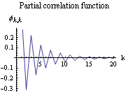
The analytic expression for the partial correlation function is _{k, k}=-(-)^k(1-²)/(1-^2(k+1)), and we see that there is no sharp cutoff in the partial correlation. This property is, in fact, shared by all the MA(q) and ARMA(p, q) models with q≠0. It can be understood by expanding an invertible MA model as an AR() model. X_t is always related to X_t-k with the intervening variables fixed for all k. Observe the duality between the AR and MA models: for an AR(p) model, the partial correlation function _{k, k} is zero for k>p and the correlation function does not have a sharp cutoff, whereas for an MA(q) model the correlation function (k) is zero for k>q and the partial correlation function has no sharp cutoff.