1.9.3 Applications of the Kalman FilterThe Kalman filtering technique can be used conveniently in the analysis of certain time series, once we write the time series model in a state-space form. In the following we will mention a few applications of the Kalman filter and illustrate some of them by examples. For a detailed treatment of the Kalman filter see, for example, Harvey (1989), Chapter 3. The simple local level model ( 9.5) is in fact in the state-space form already with Xt= t t, Gt=1, Ft=1, ct=0, and dt=0. It is easy to see that the local linear trend model ( 9.4) can be written in the state-space form as Similarly, the basic structural model (( 9.1) to ( 9.3)) when s=4 is equivalent to ARMA models can also be cast into a state-space form, which in general is nonunique. For example, one particular representation of the AR(2) model in state-space form is (for the state-space form of an ARMA( p, q) model see Harvey (1989), Chapter 3) An alternative representation for the state vector is Initializing the Kalman FilterThe initial values of  and Pt t-1 t-1 have to be given in order to start the Kalman filter. If the coefficients in ( 9.7) are all time independent and the eigenvalues of the transition matrix F are inside the unit circle, the state vector is stationary and the initial value  can be solved as and P1 0 0 obtained from The solution to the above equation is where vec( P) is the vector obtained by stacking the columns of P one below the other. For example, the AR(2) model with  1=0.9 1=0.9,  2=-0.5 2=-0.5, and  2=1 2=1 is stationary and the initial values are  and P can be obtained using ( 9.14). The following Mathematica program solves for P. getP solves for the initial value P1 0 0 for a stationary state equation. Note that Q is always symmetric. This gives P1 0 0 which is used to start the Kalman filter recursion. | Out[3]= |  |
Consider the case when the state equation is not stationary, and we do not have any prior information about the distribution of the state vector. In general, if the dimension of X is m, we can use the first m values of Y (assuming that Y is a scalar) to calculate  and Pm+1 m m and start the recursion from there. To obtain  and Pm+1 m m, we can use the Kalman filter (( 9.8) to ( 9.11)) with E(X1 I0)=E(X1)="0" I0)=E(X1)="0" and the so-called diffuse prior P1 0= 0= I I, where I is an identity matrix and  is eventually set to infinity. For example, the local level model is not stationary. In the absence of any prior information, we use  and P1 0=k 0=k and  and P2 1 1 can be obtained as follows. This gives  . Note that the result depends on the first data point y1. | Out[4]= |  |
Now we take the limit k→ . Note that we get a finite result, and the first two elements will be used as the initial values to start the recursion. | Out[5]= |  |
For the local linear trend model, X is a two-dimensional vector ( m=2), and the calculation of the initial values using a diffuse prior, in general, needs the first two data points y1 and y2. This gives  . Note that P2 1 1 is infinite, whereas P3 2 2 is finite. | Out[7]= |  |
Here  is extracted, and it can be used as the initial value to start the Kalman filter recursion. | Out[8]= |  |
Although in principle KalmanFilter can be used to calculate  using the first m data points as illustrated above, it is infeasible when m is large because of the symbolic parameter k involved in the calculation. Alternatively, we can obtain the initial values by writing Xm in terms of first m data points of Y, and therefore, solve for  . The following is a program that gives  . Note that the program is only for the case where Y is a scalar and the coefficient matrices are independent of time. For other ways of calculating starting values, see Harvey (1989), Chapter 3. This yields  given the known matrices and vectors of a state model and the first m values of data. Note that the first argument contains the first m values of the data, F and Q are m m m matrices, and G is a 1 m m matrix. When m=1, every input argument is a scalar. For example, this gives the same initial values for the local linear trend model as above but is much faster. | Out[11]= |  |
Kalman Filtering and Kalman SmoothingOften, the state variable X represents some quantity we are interested in knowing. The Kalman filter enables us to estimate the state variable X from the observations of Y. For example, in the local level model,  is the trend and the estimation of  t t, given y1, y2, ..., yt, is given by the Kalman filter ( 9.8) to ( 9.11). Example 9.1 To illustrate the use of the Kalman filter, we generate a series according to the local level model ( 9.5) with R=E 2=0.5 2=0.5 and Q=E 2=1 2=1. This generates a time series of length 100 according to the local level model ( 9.5). | Out[13]= |  |
As illustrated earlier, these are  and P2 1 1 and they are used as the starting values for KalmanFilter. | Out[14]= |  |
Using getInit we get the same result. | Out[15]= |  |
kf contains the result of the Kalman filtering. (Note that we have suppressed the output.) Note that y1 is used to obtain the initial values, so the data now starts from y2. From the Kalman filter result kf, we extract  , the estimated values of  . Here the estimate of  t t given {y1, y2, ..., yt} is plotted as a function of t. | Out[18]= | 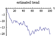 |
Xt t t is the estimate of Xt based on the information up to t. However, if we know Yt up to t=T, we can use the information up to T to improve our estimate of Xt. This is called Kalman smoothing. This gives the Kalman smoothing result. The smoothed values are plotted. | Out[20]= | 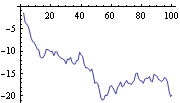 |
Example 9.2 As a second example, we use the Kalman filter to estimate the trend and the cyclic component in a particular case of the basic structural model given in ( 9.1) to ( 9.3). This generates a time series of length 100 from the basic structural model. (See 9.1 to 9.3.) The series is plotted here. | Out[22]= | 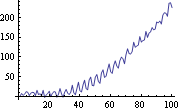 |
Various matrices that are needed are defined. Since m=5, the first five points of data y are needed to calculate the initial values. | Out[24]= |  |
This gives the Kalman filtering result. Note that the numerical value of init is used to speed up the calculation. The first component of  is the estimated trend  . The trend is extracted and plotted. | Out[26]= | 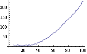 |
Similarly, the third component of  is the estimated seasonal  . Its plot is shown here. | Out[27]= | 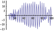 |
This gives the smoothed estimates of the state variables and their mean square errors. Here is the plot of the smoothed trend. | Out[29]= | 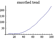 |
This is the plot of the smoothed seasonal component. | Out[30]= | 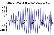 |
This gives the predicted values of the state variable for the next 15 points. We plot the smoothed trend together with the next 15 predicted values of the trend. | Out[32]= | 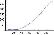 |
Here the smoothed seasonal component is plotted together with the next 15 predicted values. | Out[33]= | 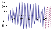 |
Parameter Estimation and PredictionThe likelihood function of a state-space time series can be easily calculated using the Kalman filter technique. The joint density of {Y1, Y2, ..., YT} is L= p(Yt p(Yt It-1) It-1), where  and  . The log likelihood is given by Note that if the first m values of data are used to calculate the starting values, the lower limit of the summations is t=m+1 and the corresponding "Log"L is the conditional log likelihood, conditional on y1, y2, ..., ym being fixed. If you wish to get the logarithm of the likelihood function of a state-space time series, you can use the function LogLikelihood[data, init, F, G, Q, R, c, d] Note that it has the same input arguments as those of KalmanFilter. When the first m points of the series are used to calculate the initial values init, data should start from ym+1; when any one of F, G, Q, R, c, d is time dependent, the above arguments to LogLikelihood, F, G, Q, R, c, d, should be replaced by {Fm+2, Fm+3, ..., FT+1}, {Gm+1, Gm+2, ..., GT}, etc. Again, if c=0 and d=0, the last two arguments can be omitted. Example 9.3 We again look at the local level model (see Example 9.1). This time we try to estimate the variance parameters of the model from the given series. We generate a time series of length 300 according to the local level model ( 9.5). This gives the initial values. Note that the parameters to be estimated should be in symbolic form. | Out[35]= |  |
To get the maximum likelihood estimate of the parameters, we need to maximize the likelihood function. This is done using the built-in Mathematica function FindMinimum. Note that the function to be minimized is the negative of the log likelihood function. Also, we define a special function which evaluates only for numerical input to prevent FindMinimum from attempting symbolic preprocessing that can potentially take a long time. | Out[39]= |  |
Example 9.4 Here we give another example using the local linear trend model. We generate a series from the local linear trend model. The initial values depend on the parameters  ,  , and  , which are to be estimated. | Out[42]= |  |
This gives the estimate of the parameters. | Out[46]= |  |
Having obtained the estimated parameters, we can now use them to predict the future trend  by using KalmanPredictor. First, we calculate {Xt+1 t, Pt+1 t, Pt+1 t} t} from KalmanFilter. We substitute the estimated parameters. | Out[48]= |  |
These are the values of {Xt+1 t, Pt+1 t, Pt+1 t} t}. | Out[49]= |  |
This gives the next 20 predicted values of X and their mean square errors. The predicted trend is given by the first component of X. | Out[51]= |  |
This shows the predicted trend along with the given series. | Out[52]= | 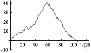 |
Example 9.5 As a final example, we look at the AR(2) model and show that the Kalman filter approach gives the same estimation of parameters as the method introduced in the previous sections. This generates an AR(2) series of length 50. This gives the initial P1 0 0. | Out[54]= |  |
FindMinimum finds the parameter values that maximize the likelihood function. | Out[58]= |  |
We can get the same result using MLEstimate. Note that for the one-dimensional ARMA model, the concentrated likelihood is calculated. Therefore, the variance q should not be included as a search parameter. | Out[59]= |  |
Note that the value of the log likelihood is different from that obtained using the Kalman filter. This is because the former calculates the concentrated likelihood whereas the latter, the full likelihood (apart from a constant). | Out[60]= |  |
On the other hand, had we used the first two data points to calculate the initial values, we would have effectively obtained the conditional maximum likelihood estimate, conditional on the first two data points being fixed. The initial values obtained this way correspond to using a diffuse prior. | Out[61]= |  |
This gives the estimated parameters. | Out[65]= |  |
We can get the same result much faster using ConditionalMLEstimate. | Out[67]= |  |
|