Contactless Anemometer

In this application a contactless fluid flow anemometer is simulated. We present a microelectromechanical system (MEMS) device that can be attached to a pipe and measure a fluid flow velocity that is present in the pipe in a contact less manner [1, 2]. To achieve this, a small section in the device is heated and a flow passing over the heater will distort the temperature profile generated by the heater. The distortion of the temperature profile can then be measured by thermal sensors at two points and from the difference in temperature the velocity of the fluid passing the device can be computed.

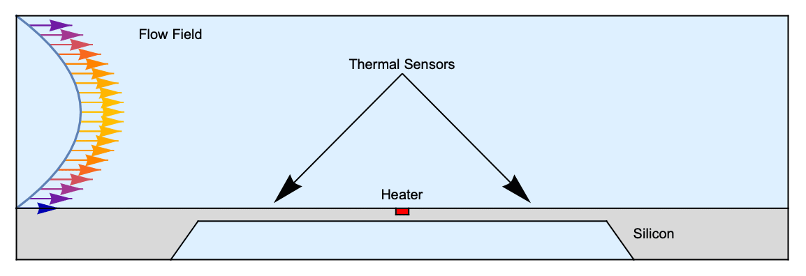
The figure shows a sketch of the anemometer device. The device is shown in gray and made of silicon. A small heater, shown in red, also made of silicon, is embedded. A fluid passes over the device from left to right. The blue part below is the same fluid but no flow field is present in that section. Two thermal sensors are embedded to the left and right of the heater. Once a flow field passes over the heater the heat profile will be asymmetrical and a temperature difference between the two thermal sensors can be detected.

Load the Finite Element package:

Model

To model the device a heat transfer simulation is performed. The heat equation is given by:

where is the temperature distribution, the mass density, , the specific heat capacity, the thermal conductivity, the fluid flow velocity and a heat source. All coefficients will have different values in different material regions in the simulation domain. The thermal conductivity is a diffusion coefficient and is active in the entire simulation domain, however, different values apply in different regions. is a convection coefficient and is only active where the fluid is flowing over the device. is a load coefficient and will be used to model the heater in the device.

Set up time independent variables:

Mesh generation

We start by manually setting up a boundary geometry. First some device parameters like sizes and angles are set up.

Set up a scale:

Set up geometric parameters:

is the angle for the cut out in the silicon device.

Additional geometric parameters:

The coordinates for the boundary mesh:

Group the coordinates together:

Create the boundary segments that provide the information how the coordinates are connected:

Group the segments:

Visualize a graphics of the device:

Now, that we have coordinates of the boundary geometry markers are added to facilitate the application of boundary conditions and different material parameters in the device. A detailed introduction to markers is given in a section about markers in the ElementMesh generation tutorial.

Set up boundary markers:

Group the markers:

Set up the point element incidents and markers:

Create the boundary mesh:

Inspect the point markers:

Inspect the boundary markers:

Now, that a boundary mesh is set up the full mesh is constructed. The boundary mesh is augmented with region markers. These are specified by a coordinate point inside the respective sub-region, an integer marker and a specification for the amount of refinement in that sub-region.

Generate coordinates in the different sub-regions:

Visualize the marker coordinates in the boundary mesh:

Generate the full mesh with region markers and specified mesh element refinement sizes:

Visualize the mesh with air in blue, silicon in gray and the heater in read:

All in all, we have four different parts in the simulation domain. The silicon device as such, the heater, the flow region and the cut out underneath the silicon. The material data for the silicon and the heater is the same and so is fluid above and below the silicon.

Inspect the region markers:

Visualize the part of the mesh that has ElementMarker set to 1:

Material and model

Next the material data is set up. The device is made of silicon and as a fluid we use air. The material data will have different values in different sub-regions of the device.

Setup the thermal conductivity:

Set up the convection:

Plot the convection flow profile:

Visualize the flow field above the silicon:

Set up the load:

Set up the mass density of the sub-regions:

Set up the specific heat capacity of the sub-regions:

Set up the parameters and the model:

We set a temperature at the lower edge of the simulation domain.

Show the positions of the HeatTemperatureCondition:

Set up the boundary conditions:

Solve the partial differential equation:

Visualize the solution:

Compute the minimum and maximum temperatures:

Compute the temperature difference between to points on the device:

As a next step, we would like to inspect the dynamic behaviour of the device.

Set up time variables:

Regenerate the partial differential equation:

Re set up the boundary conditions:

Additionally an initial condition needs to be specified, here we start from a zero temperature:

Set up an initial condition:

Solve the partial differential equation:

Find the minimal and maximal solution values:

Create contour plots at various times:

To obtain high quality graphics remove or comment out the call to Rasterize.

Animate the dynamics of the contact less heat anemometer:

From this we can see that placing the thermal sensor that is to the left of the heat even further to the left would result in a higher temperature difference.

References

1. Ernst, Herbert; High-Resolution Thermal Measurements in Fluids; PhD thesis; Universität Freiburg, 2001: https://freidok.uni-freiburg.de/fedora/objects/freidok:201/datastreams/FILE1/content

2. Rübenkönig, Oliver; Free Surface Flow and the IMTEK Mathematica Supplement; PhD thesis; Universität Freiburg, 2008: https://freidok.uni-freiburg.de/data/6440

Top