ListStreamPlot3D
ListStreamPlot3D[varr]
plots streamlines for the vector field given as an array of vectors.
Details and Options
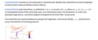
- ListStreamPlot3D is known as a 3D stream plot or streamline plot. Besides lines, streamlines can also be displayed as tubes (stream tubes) and ribbons (stream ribbons).
- ListStreamPlot3D plots streamlines
 defined by
  and
and  where
where  is an interpolated function of the vector data and
  is an initial stream point. The streamline
  is the curve passing through point
  , and whose tangents correspond to the vector field
  at each point.
 - The streamlines are colored by default according to the magnitude
 of the vector field
  and have an arrow in the direction of increasing value of
  .
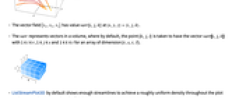
. - The vector field
 has value varr〚i,j,k〛 at
  .
. - The varr represents vectors in a volume, where by default, the point {k,j,i} is taken to have the vector varr〚i,j,k〛 with 1≤i≤r, 1≤j≤s and 1≤k≤t for an array of dimension {r,s,t,3}.
- ListStreamPlot3D by default shows enough streamlines to achieve a roughly uniform density throughout the plot and shows no background scalar field.
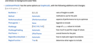
- ListStreamPlot3D has the same options as Graphics3D, with the following additions and changes: [List of all options]
-
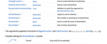
BoxRatios {1,1,1} ratio of height to width Method Automatic methods to use for the plot PerformanceGoal $PerformanceGoal aspects of performance to try to optimize PlotLegends None legends to include PlotRange {Full,Full,Full} range of x, y, z values to include PlotRangePadding Automatic how much to pad the range of values PlotTheme $PlotTheme overall theme for the plot RegionBoundaryStyle Automatic how to style plot region boundaries RegionFunction True& determine what region to include ScalingFunctions None how to scale individual coordinates StreamColorFunction Automatic how to color streamlines StreamColorFunctionScaling True whether to scale the argument to StreamColorFunction StreamMarkers Automatic shape to use for streams StreamPoints Automatic the number or placement of streamlines StreamScale None how to scale the sizes of streamlines StreamStyle Automatic how to draw streamlines - The arguments supplied to functions in RegionFunction and ColorFunction are x,y,z,vx,vy,vz,Norm[{vx,vy,vz}].
- Possible settings for StreamMarkers include:
-
"Arrow" lines with 2D arrowheads 
"Arrow3D" tubes with 3D arrowheads 
"Line" lines 
"Tube" tubes 
"Ribbon" flat ribbons 
"ArrowRibbon" ribbons with built-in arrowheads - With StreamScaleAutomatic and "arrow" stream markers, the streamlines are split into segments to make it easier to see the direction of the streamlines.
- Possible settings for StreamScale are:
-
Automatic automatically determine the streamline segments Full show the streamline as one piece Tiny,Small,Medium,Large named settings for how long the segments should be {len,npts,ratio} use explicit specification of streamline segmentation - The length len of streamline segments can be one of the following forms:
-
Automatic automatically determine the length None show the streamline as one piece Tiny,Small,Medium,Large use named segment lengths s use a length s that is a fraction of the graphic size - The number of points npts used to draw each segment can be Automatic or a specific number of points.
- The aspect ratio ratio specifies how wide the cross section of a streamline is relative to the streamline segment.
- Possible settings for ScalingFunctions are:
-
{sx,sy,sz} scale x, y and z axes - Common built-in scaling functions s include:
-
"Log" 
log scale with automatic tick labeling "Log10" 
base-10 log scale with powers of 10 for ticks "SignedLog" 
log-like scale that includes 0 and negative numbers "Reverse" 
reverse the coordinate direction "Infinite" 
infinite scale -
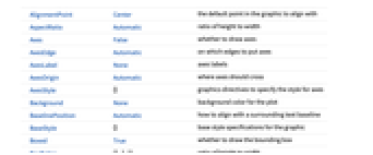
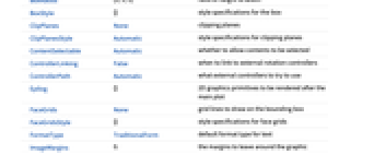
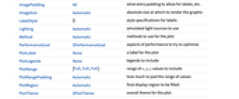
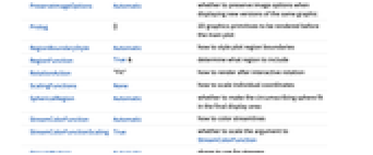
AlignmentPoint Center the default point in the graphic to align with AspectRatio Automatic ratio of height to width Axes False whether to draw axes AxesEdge Automatic on which edges to put axes AxesLabel None axes labels AxesOrigin Automatic where axes should cross AxesStyle {} graphics directives to specify the style for axes Background None background color for the plot BaselinePosition Automatic how to align with a surrounding text baseline BaseStyle {} base style specifications for the graphic Boxed True whether to draw the bounding box BoxRatios {1,1,1} ratio of height to width BoxStyle {} style specifications for the box ClipPlanes None clipping planes ClipPlanesStyle Automatic style specifications for clipping planes ContentSelectable Automatic whether to allow contents to be selected ControllerLinking False when to link to external rotation controllers ControllerPath Automatic what external controllers to try to use Epilog {} 2D graphics primitives to be rendered after the main plot FaceGrids None grid lines to draw on the bounding box FaceGridsStyle {} style specifications for face grids FormatType TraditionalForm default format type for text ImageMargins 0. the margins to leave around the graphic ImagePadding All what extra padding to allow for labels, etc. ImageSize Automatic absolute size at which to render the graphic LabelStyle {} style specifications for labels Lighting Automatic simulated light sources to use Method Automatic methods to use for the plot PerformanceGoal $PerformanceGoal aspects of performance to try to optimize PlotLabel None a label for the plot PlotLegends None legends to include PlotRange {Full,Full,Full} range of x, y, z values to include PlotRangePadding Automatic how much to pad the range of values PlotRegion Automatic final display region to be filled PlotTheme $PlotTheme overall theme for the plot PreserveImageOptions Automatic whether to preserve image options when displaying new versions of the same graphic Prolog {} 2D graphics primitives to be rendered before the main plot RegionBoundaryStyle Automatic how to style plot region boundaries RegionFunction True& determine what region to include RotationAction "Fit" how to render after interactive rotation ScalingFunctions None how to scale individual coordinates SphericalRegion Automatic whether to make the circumscribing sphere fit in the final display area StreamColorFunction Automatic how to color streamlines StreamColorFunctionScaling True whether to scale the argument to StreamColorFunction StreamMarkers Automatic shape to use for streams StreamPoints Automatic the number or placement of streamlines StreamScale None how to scale the sizes of streamlines StreamStyle Automatic how to draw streamlines Ticks Automatic specification for ticks TicksStyle {} style specification for ticks TouchscreenAutoZoom False - whether to zoom to fullscreen when activated on a touchscreen
ViewAngle Automatic angle of the field of view ViewCenter Automatic point to display at the center ViewMatrix Automatic explicit transformation matrix ViewPoint {1.3,-2.4,2.} viewing position ViewProjection Automatic projection method for rendering objects distant from the viewer ViewRange All range of viewing distances to include ViewVector Automatic position and direction of a simulated camera ViewVertical {0,0,1} direction to make vertical
List of all options
Examples
open allclose allBasic Examples (4)
Scope (12)
Sampling (3)
Presentation (9)
Streamlines are drawn as lines by default:
Use 3D tubes for the streamlines:
Use "arrow" versions of the stream markers to indicate the direction of flow along the streamlines:
Ribbons are turned into arrows by tapering the heads and notching the tails of the streamlines:
Use a single color for the streamlines:
Use a named color gradient for the streamlines:
Include a legend for the field magnitude:
Use StreamScale to split streamlines into multiple shorter line segments:
Increase the number of points in each segment and increase the marker aspect ratio:
Options (46)
BoxRatios (2)
DataRange (2)
PlotLegends (3)
RegionBoundaryStyle (4)
Show the region defined by a RegionFunction:
Use None to avoid showing the boundary:
RegionFunction (4)
Plot streamlines in a restricted region:
Plot streams only where the field magnitude exceeds a given threshold:
Region functions depend, in general, on seven arguments:
Use RegionBoundaryStyleNone to avoid showing the boundary:
ScalingFunctions (3)
StreamColorFunction (4)
Color the streams by their norm:
Use any named color gradient from ColorData:
Color the streamlines according to their x value:
Use StreamColorFunctionScalingFalse to get unscaled values:
StreamColorFunctionScaling (2)
StreamMarkers (5)
StreamPoints (4)
StreamScale (9)
Segmented markers have default lengths, numbers of points and aspect ratios:
Modify the lengths of the segments:
Specify the number of sample points in each segment:
Modify the aspect ratios for the stream markers:
Make segmented markers continuous:
Break continuous markers into segments:
The aspect ratio controls the thickness of ribbons and tubes:
StreamStyle (3)
Change the appearance of the streamlines:
StreamColorFunction takes precedence over StreamStyle:
Use StreamColorFunctionNone to specify a streamline color with StreamStyle:
Applications (2)
Numerically compute the electric field at a sampling of points under the influence of two thin wires of finite length with equal constant charge densities and opposite signs:
Visualize the electric field along with the positively charged (black) and the negatively charged (red) wires:
Visualize time-independent heat flow in a unit cube. Consider the steady-state heat equation ![]() for the temperature
for the temperature ![]() on the unit cube with
on the unit cube with ![]() on the
on the ![]() face, insulated on the
face, insulated on the ![]() ,
, ![]() ,
, ![]() and
and ![]() faces,
faces, ![]() inside a centered disk of radius 0.3 on the
inside a centered disk of radius 0.3 on the ![]() face and
face and ![]() outside the disk as shown in the following:
outside the disk as shown in the following:
Use finite differences to discretize the heat equation ![]() :
:
Specify boundary conditions for ![]() on the
on the ![]() and
and ![]() faces:
faces:
Specify the insulated boundary conditions for ![]() on the other faces:
on the other faces:
Solve the system of equations:
Use finite differences to approximate the heat flux:
Generate seed points for the streamlines on the ![]() face:
face:
Generate seed points for the streamlines in the red disk on the ![]() face:
face:
Visualize the heat flow. The boundary temperatures are specified in the legend, and the blank faces of the cube are insulated:
Properties & Relations (10)
Use StreamPlot3D and VectorPlot3D to visualize functions:
Use StreamPlot and VectorPlot to visualize functions in 2D:
Plot vectors along surfaces with ListSliceVectorPlot3D:
Use ListVectorPlot3D to plot a 3D field as discrete vectors:
Use ListVectorPlot for plotting 2D vectors:
Use ListStreamPlot to plot with streamlines instead of vectors:
Use ListVectorDensityPlot or ListStreamDensityPlot to add a density plot of a scalar field:
Use ListVectorDisplacementPlot to visualize the deformation of a region associated with a displacement vector field:
Use ListVectorDisplacementPlot3D to visualize a deformation in 3D:
Use ListLineIntegralConvolutionPlot to plot the line integral convolution of a vector field:
Use GeoVectorPlot to plot vectors on a map:
Use GeoStreamPlot to plot streamlines instead of vectors:
Possible Issues (2)
Tube StreamMarkers can be distorted by the BoxRatios:
Carefully adjusting the BoxRatios can eliminate the tube distortion:
The colors of "Arrow" and "Arrow3D" stream markers are determined at the tip of the arrow, which can result in inconsistent colors for long arrows:
Text
Wolfram Research (2021), ListStreamPlot3D, Wolfram Language function, https://reference.wolfram.com/language/ref/ListStreamPlot3D.html (updated 2022).
CMS
Wolfram Language. 2021. "ListStreamPlot3D." Wolfram Language & System Documentation Center. Wolfram Research. Last Modified 2022. https://reference.wolfram.com/language/ref/ListStreamPlot3D.html.
APA
Wolfram Language. (2021). ListStreamPlot3D. Wolfram Language & System Documentation Center. Retrieved from https://reference.wolfram.com/language/ref/ListStreamPlot3D.html