Numerical Solution of Boundary Value Problems (BVP)
"Shooting" Method
The shooting method works by considering the boundary conditions as a multivariate function of initial conditions at some point, reducing the boundary value problem to finding the initial conditions that give a root. The advantage of the shooting method is that it takes advantage of the speed and adaptivity of methods for initial value problems. The disadvantage of the method is that it is not as robust as finite difference or collocation methods: some initial value problems with growing modes are inherently unstable even though the BVP itself may be quite well posed and stable.
The shooting method looks for initial conditions ![]() so that
so that ![]() . Since you are varying the initial conditions, it makes sense to think of
. Since you are varying the initial conditions, it makes sense to think of ![]() as a function of them, so shooting can be thought of as finding
as a function of them, so shooting can be thought of as finding ![]() such that
such that
After setting up the function for ![]() , the problem is effectively passed to FindRoot to find the initial conditions
, the problem is effectively passed to FindRoot to find the initial conditions ![]() giving the root. The default method is to use Newton's method, which involves computing the Jacobian. While the Jacobian can be computed using finite differences, the sensitivity of solutions of an initial value problem (IVP) to its initial conditions may be too much to get reasonably accurate derivative values, so it is advantageous to compute the Jacobian as a solution to ODEs.
giving the root. The default method is to use Newton's method, which involves computing the Jacobian. While the Jacobian can be computed using finite differences, the sensitivity of solutions of an initial value problem (IVP) to its initial conditions may be too much to get reasonably accurate derivative values, so it is advantageous to compute the Jacobian as a solution to ODEs.
Linearization and Newton's Method
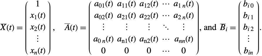
Linear problems can be described by
where ![]() is a matrix and
is a matrix and ![]() is a vector both possibly depending on
is a vector both possibly depending on ![]() ,
, ![]() is a constant vector, and
is a constant vector, and ![]() are constant matrices.
are constant matrices.
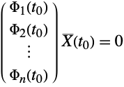
Let ![]() . Then, differentiating both the IVP and boundary conditions with respect to
. Then, differentiating both the IVP and boundary conditions with respect to ![]() gives
gives
Since ![]() is linear, when thought of as a function of
is linear, when thought of as a function of ![]() , you have
, you have ![]() , so the value of
, so the value of ![]() for which
for which ![]() satisfies
satisfies
for any particular initial condition ![]() .
.
For nonlinear problems, let ![]() be the Jacobian for the nonlinear ODE system, and let
be the Jacobian for the nonlinear ODE system, and let ![]() be the Jacobian of the
be the Jacobian of the ![]() th boundary condition. Then computation of
th boundary condition. Then computation of ![]() for the linearized system gives the Jacobian for the nonlinear system for a particular initial condition, leading to a Newton iteration,
for the linearized system gives the Jacobian for the nonlinear system for a particular initial condition, leading to a Newton iteration,
"StartingInitialConditions"
For boundary value problems, there is no guarantee of uniqueness as there is in the initial value problem case. "Shooting" will find only one solution. Just as you can affect the particular solution FindRoot gets for a system of nonlinear algebraic equations by changing the starting values, you can change the solution that "Shooting" finds by giving different initial conditions to start the iterations from.
"StartingInitialConditions" is an option of the "Shooting" method that allows you to specify the values and position of the initial conditions to start the shooting process from.
The shooting method by default starts with zero initial conditions so that if there is a zero solution, it will be returned.
sols = Map[First[NDSolve[{x''[t] + Sin[x[t]] == 0, x[0] == x[10] == 0}, x, t, Method -> {"Shooting", "StartingInitialConditions" -> {x[0] == 0, x'[0] == #}}]]&,
	{1.5, 1.75, 2}];
Plot[Evaluate[x[t] /. sols], {t, 0, 10}, PlotStyle -> {StandardBrown, StandardBlue, StandardGreen}]
By default, "Shooting" starts from the left side of the interval and shoots forward in time. There are cases where it is advantageous to go backward, or even from a point somewhere in the middle of the interval.
Consider the linear boundary value problem
For moderate values of ![]() , the initial value problem starting at
, the initial value problem starting at ![]() becomes unstable because of the growing
becomes unstable because of the growing ![]() and
and ![]() terms. Similarly, starting at
terms. Similarly, starting at ![]() , instability arises from the
, instability arises from the ![]() term, though this is not as large as the term in the forward direction. Beyond some value of
term, though this is not as large as the term in the forward direction. Beyond some value of ![]() , shooting will not be able to get a good solution because the sensitivity in either direction will be too great. However, up to that point, choosing a point in the interval that balances the growth in the two directions will give the best solution.
, shooting will not be able to get a good solution because the sensitivity in either direction will be too great. However, up to that point, choosing a point in the interval that balances the growth in the two directions will give the best solution.
eqn = x'''[t] - 2λ x''[t] - λ^2x'[t] + 2λ^3x[t] == (λ^2 + π^2) (2 λ Cos[π t] + π Sin[π t]);
bcs = {x[0]  ==   1 + (1 + E^-2 λ + E^-λ/2 + E^-λ), x[1] == 0, x'[1] == (3 λ - E^-λ λ/2 + E^-λ)};
xsol[t_] = (E^λ (t - 1) + E^2 λ (t - 1) + E^-λ t/2 + E^-λ) + Cos[π t];Block[{λ = 10},
sol = First[NDSolve[{eqn, bcs}, x, t]];
Plot[{xsol[t], x[t] /. sol}, {t, 0, 1}]]Shooting from ![]() , the "Shooting" method gives warning messages about an ill-conditioned matrix and that the boundary conditions are not satisfied as well as they should be. This is because a small error at
, the "Shooting" method gives warning messages about an ill-conditioned matrix and that the boundary conditions are not satisfied as well as they should be. This is because a small error at ![]() is amplified by
is amplified by ![]() Since the reciprocal of this is of the same order of magnitude as the local truncation error, visible errors such as those seen in the plot are not surprising. In the reverse direction, the magnification will be much less:
Since the reciprocal of this is of the same order of magnitude as the local truncation error, visible errors such as those seen in the plot are not surprising. In the reverse direction, the magnification will be much less: ![]() , so the solution should be much better.
, so the solution should be much better.
Block[{λ = 10},
	sol = First[NDSolve[{eqn, bcs}, x, t,
	Method -> {"Shooting", "StartingInitialConditions" -> {x[1] == 0, x'[1] == (3 λ - E^-λ λ/2 + E^-λ), x''[1] == 0}}]];
	Plot[{xsol[t], x[t] /. sol}, {t, 0, 1}]]
A good point to choose is one that will balance the sensitivity in each direction, which is about at ![]() . With this, the error with
. With this, the error with ![]() will still be under reasonable control.
will still be under reasonable control.
Block[{λ = 15},
	sol = First[NDSolve[{eqn, bcs}, x, t,
	Method -> {"Shooting", "StartingInitialConditions" -> {x[2 / 3] == 0, x'[2 / 3] == 0, x''[2 / 3] == 0}}]];
	Plot[{xsol[t], x[t] /. sol}, {t, 0, 1}]]
Option Summary
option name | default value | |
| "StartingInitialConditions" | Automatic | the initial conditions to initiate the shooting method from |
| "ImplicitSolver" | Automatic | the method to use for solving the implicit equation defined by the boundary conditions; this should be an acceptable value for the Method option of FindRoot |
| "MaxIterations" | Automatic | how many iterations to use for the implicit solver method |
| "Method" | Automatic | the method to use for integrating the system of ODEs |
"Chasing" Method
The method of chasing came from a manuscript of Gelfand and Lokutsiyevskii first published in English in [BZ65] and further described in [Na79]. The idea is to establish a set of auxiliary problems that can be solved to find initial conditions at one of the boundaries. Once the initial conditions are determined, the usual methods for solving initial value problems can be applied. The chasing method is, in effect, a shooting method that uses the linearity of the problem to good advantage. As such, the chasing method can be used for linear differential equations.
where ![]() ,
, ![]() is the coefficient matrix, and
is the coefficient matrix, and ![]() is the inhomogeneous coefficient vector, with
is the inhomogeneous coefficient vector, with ![]() linear boundary conditions
linear boundary conditions
where ![]() is a coefficient vector. From this, construct the augmented homogeneous system
is a coefficient vector. From this, construct the augmented homogeneous system
The chasing method amounts to finding a vector function ![]() such that
such that ![]() and
and ![]() . Once the function
. Once the function ![]() is known, if there is a full set of boundary conditions, solving
is known, if there is a full set of boundary conditions, solving
can be used to determine initial conditions ![]() that can be used with the usual initial value problem solvers. Note that the solution to system (3) is nontrivial because the first component of
that can be used with the usual initial value problem solvers. Note that the solution to system (3) is nontrivial because the first component of ![]() is always 1.
is always 1.
Thus, solving the boundary value problem is reduced to solving the auxiliary problems for the ![]() . Differentiating the equation for
. Differentiating the equation for ![]() gives
gives
substituting the differential equation,
Since this should hold for all solutions ![]() , you have the initial value problem for
, you have the initial value problem for ![]() ,
,
Given ![]() where you want to have solutions to all of the boundary value problems, the Wolfram Language just uses NDSolve to solve the auxiliary problems for
where you want to have solutions to all of the boundary value problems, the Wolfram Language just uses NDSolve to solve the auxiliary problems for ![]() by integrating them to
by integrating them to ![]() . The results are then combined into the matrix of (3) that is solved for
. The results are then combined into the matrix of (3) that is solved for ![]() to obtain the initial value problem that NDSolve integrates to give the returned solution.
to obtain the initial value problem that NDSolve integrates to give the returned solution.
This variant of the method is further described in and used by the MathSource package [R98], which also allows you to solve linear eigenvalue problems.
There is an alternative, nonlinear way to set up the auxiliary problems that is closer to the original method proposed by Gelfand and Lokutsiyevskii. Assume that the boundary conditions are linearly independent (if not, then the problem is insufficiently specified). Then in each ![]() , there is at least one nonzero component. Without loss of generality, assume that
, there is at least one nonzero component. Without loss of generality, assume that ![]() . Now solve for
. Now solve for ![]() in terms of the other components of
in terms of the other components of ![]() ,
, ![]() , where
, where ![]() and
and ![]() . Using (5) and replacing
. Using (5) and replacing ![]() , and thinking of
, and thinking of ![]() in terms of the other components of
in terms of the other components of ![]() , you get the nonlinear equation
, you get the nonlinear equation
where ![]() is
is ![]() with the
with the ![]() thcolumn removed, and
thcolumn removed, and ![]() is the
is the ![]() th column of A. The nonlinear method can be more numerically stable than the linear method, but it has the disadvantage that integration along the real line may lead to singularities. This problem can be eliminated by integrating on a contour in the complex plane. However, the integration in the complex plane typically has more numerical errors than a simple integration along the real line, so in practice, the nonlinear method does not typically give results better than the linear method. For this reason, and because it is also generally faster, the default for the Wolfram Language is to use the linear method.
th column of A. The nonlinear method can be more numerically stable than the linear method, but it has the disadvantage that integration along the real line may lead to singularities. This problem can be eliminated by integrating on a contour in the complex plane. However, the integration in the complex plane typically has more numerical errors than a simple integration along the real line, so in practice, the nonlinear method does not typically give results better than the linear method. For this reason, and because it is also generally faster, the default for the Wolfram Language is to use the linear method.
nsol1 = NDSolve[{y''[t] + y[t] / 4 == 8, y[0] == 0, y[10] == 0}, y, {t, 0, 10}]Plot[First[y[t] /. nsol1], {t, 0, 10}]bconds = {
x[0] + x'[0] + y[0] + y'[0] == 1,
x[1] + 2 x'[1] + 3 y[1] + 4y'[1] == 5,
y[2] + 2 y'[2] == 4,
x[3] - x'[3] == 7};
nsol2 = NDSolve[{
x''[t] + x[t] + y[t] == t, y''[t] + y[t] == Cos[t],
bconds},
{x, y},
{t, 0, 4}]In general, you cannot expect the boundary value equations to be satisfied to the close tolerance of Equal.
bconds /. First[nsol2]They are typically only satisfied at most tolerances that come from the AccuracyGoal and PrecisionGoal options of NDSolve. Usually, the actual accuracy and precision is less because these are used for local, not global, error control.
Apply[Subtract, bconds, 1] /. First[nsol2]When you give NDSolve a problem that has no solution, numerical error may make it appear to be a solvable problem. Typically, NDSolve will issue a warning message.
NDSolve[{x''[t] + x[t] == 0, x[0] == 1, x[Pi] == 0}, x, {t, 0, Pi}, Method -> "Chasing"]In this case, it is not able to integrate over the entire interval because of nonexistence.
Another situation in which the equations can be ill-conditioned is when the boundary conditions do not give a unique solution.
dsol = First[x /. DSolve[{x''[t] + x[t] == t, x'[0] == 1, x[Pi / 2] == Pi / 2}, x, t]]onesol = First[x /. NDSolve[{x''[t] + x[t] == t, x'[0] == 1, x[Pi / 2] == Pi / 2}, x, {t, 0, Pi / 2}, Method -> "Chasing"]]ip = onesol@"Coordinates"[1];
points = Transpose[{ip, onesol[ip]}];
model = dsol[t] /. C[1] -> α;
fit = FindFit[points, model, α, t];
ListPlot[Transpose[{ip, onesol[ip] - ((model /. fit) /. t -> ip)}]]Typically, the default values the Wolfram Language uses work fine, but you can control the chasing method by giving NDSolve the option Method->{"Chasing",chasing options}. The possible chasing options are shown in the following table.
option name | default value | |
| Method | Automatic | the numerical method to use for computing the initial value problems generated by the chasing algorithm |
| "ExtraPrecision" | 0 | number of digits of extra precision to use for solving the auxiliary initial value problems |
| "ChasingType" | "LinearChasing" | the type of chasing to use, which can be either "LinearChasing" or "NonlinearChasing" |
Options for the "Chasing" method of NDSolve.
The method "ChasingType"->"NonlinearChasing" itself has two options.
option name | default value | |
| "ContourType" | "Ellipse" | the shape of contour to use when integration in the complex plane is required, which can either be "Ellipse" or "Rectangle" |
| "ContourRatio" | 1/10 | the ratio of the width to the length of the contour; typically a smaller number gives more accurate results, but yields more numerical difficulty in solving the equations |
Options for the "NonlinearChasing" option of the "Chasing" method.
These options, especially "ExtraPrecision", can be useful in cases where there is a strong sensitivity to computed initial conditions.
bvp = {x''[t] + 1000 x[t] == 0, x[0] == 0, x[1] == 1};
dsol = First[x /. DSolve[bvp, x, t]]sol = First[x /. NDSolve[{x''[t] + 1000 x[t] == 0, x[0] == 0, x[1] == 1}, x, {t, 0, 1}, Method -> "Chasing"]];
Plot[sol[t] - dsol[t], {t, 0, 1}]sol = First[x /. NDSolve[{x''[t] + 1000 x[t] == 0, x[0] == 0, x[1] == 1}, x, {t, 0, 1}, Method -> {"Chasing", "ExtraPrecision" -> 10}]];
Plot[sol[t] - dsol[t], {t, 0, 1}]Increasing the extra precision beyond this really will not help because a significant part of the error results from computing the solution once the initial conditions are found. To reduce this, you need to give more stringent AccuracyGoal and PrecisionGoal options to NDSolve.
sol = First[x /. NDSolve[{x''[t] + 1000 x[t] == 0, x[0] == 0, x[1] == 1}, x, {t, 0, 1}, Method -> {"Chasing", "ExtraPrecision" -> 10}, AccuracyGoal -> 10, PrecisionGoal -> 10]];
Plot[sol[t] - dsol[t], {t, 0, 1}]
Boundary Value Problems with Parameters
In many of the applications where boundary value problems arise, there may be undetermined parameters, such as eigenvalues, in the problem itself that may be a part of the desired solution. By introducing the parameters as dependent variables, the problem can often be written as a boundary value problem in standard form.
For example, the flow in a channel can be modeled by
where ![]() (the Reynolds number) is given, but
(the Reynolds number) is given, but ![]() is to be determined.
is to be determined.
To find the solution ![]() and the value of
and the value of ![]() , just add the equation
, just add the equation ![]() .
.
Block[{R = 1}, sol = NDSolve[{f'''[t] - R((f'[t]) ^ 2 - f[t] f''[t]) + R a[t] == 0, a'[t] == 0, f[0] == f'[0] == f'[1] == 0, f[1] == 1}, {f, a}, t];
	Column[{Plot[f[t] /. First[sol], {t, 0, 1}],
	a[0] /. First[sol]}]]