The Design of the NDSolve Framework
| Features | Method Classes |
| Common Time Stepping | Automatic Selection and User Controllability |
| Data Encapsulation | MethodMonitor |
| Method Hierarchy | Shared Features |
| User Extensibility | Some Basic Methods |
Features
Supporting a large number of numerical integration methods for differential equations is a lot of work.
In order to cut down on maintenance and duplication of code, common components are shared between methods.
This approach also allows code optimization to be carried out in just a few central routines.
The principal features of the NDSolve framework are:
- Vectorized framework based on a generalization of the BLAS model [LAPACK99] using optimized in-place arithmetic
Common Time Stepping
A common time-stepping mechanism is used for all one-step methods. The routine handles a number of different criteria including:
- Step sizes in a numerical integration do not become too small in value, which may happen in solving stiff systems
- Rounding error feedback (compensated summation) is particularly advantageous for high-order methods or methods that conserve specific quantities during the numerical integration
Data Encapsulation
Each method has its own data object that contains information that is needed for the invocation of the method. This includes, but is not limited to, coefficients, workspaces, step-size control parameters, step-size acceptance/rejection information, and Jacobian matrices. This is a generalization of the ideas used in codes like LSODA ([H83], [P83]).
Method Hierarchy
Methods are reentrant and hierarchical, meaning that one method can call another. This is a generalization of the ideas used in the Generic ODE Solving System, Godess (see [O95], [O98], and the references therein), which is implemented in C++.
Initial Design
The original method framework design allowed a number of methods to be invoked in the solver.
NDSolve ⟶ "ExplicitRungeKutta"
NDSolve ⟶ "ImplicitRungeKutta"
First Revision
This was later extended to allow one method to call another in a sequential fashion, with an arbitrary number of levels of nesting.
NDSolve ⟶ "Extrapolation" ⟶ "ExplicitMidpoint"
The construction of compound integration methods is particularly useful in geometric numerical integration.
NDSolve ⟶ "Projection" ⟶ "ExplicitRungeKutta"
Second Revision
A more general tree invocation process was required to implement composition methods.
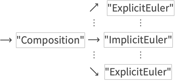
This is an example of a method composed with its adjoint.
Current State
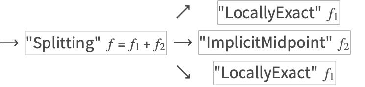
The tree invocation process was extended to allow for a subfield to be solved by each method, instead of the entire vector field.
This example turns up in the ABC Flow subsection of "Composition and Splitting Methods for NDSolve".
User Extensibility
Built-in methods can be used as building blocks for the efficient construction of special-purpose (compound) integrators. User-defined methods can also be added.
Method Classes
Methods such as "ExplicitRungeKutta" include a number of schemes of different orders. Moreover, alternative coefficient choices can be specified by the user. This is a generalization of the ideas found in RKSUITE [BGS93].
Automatic Selection and User Controllability
The framework provides automatic step-size selection and method-order selection. Methods are user-configurable via method options.
For example, a user can select the class of "ExplicitRungeKutta" methods, and the code will automatically attempt to ascertain the "optimal" order according to the problem, the relative and absolute local error tolerances, and the initial step-size estimate.
Here is a list of options appropriate for "ExplicitRungeKutta".
MethodMonitor
In order to illustrate the low-level behavior of some methods, such as stiffness switching or order variation that occurs at run time, a new "MethodMonitor" has been added.
This fits between the relatively coarse resolution of "StepMonitor" and the fine resolution of "EvaluationMonitor" .
This feature is not officially documented and the functionality may change in future versions.
Shared Features
These features are not necessarily restricted to NDSolve since they can also be used for other types of numerical methods.
- Function evaluation is performed using a NumericalFunction that dynamically changes type as needed, such as when IEEE floating-point overflow or underflow occurs. It also calls the Wolfram Language's compiler Compile for efficiency when appropriate.
- Jacobian evaluation uses symbolic differentiation or finite difference approximations, including automatic or user-specifiable sparsity detection.
- Dense linear algebra is based on LAPACK, and sparse linear algebra uses special-purpose packages such as UMFPACK.
- Common subexpressions in the numerical evaluation of the function representing a differential system are detected and collected to avoid repeated work.
- Other supporting functionality that has been implemented is described in "Norms in NDSolve".
This system dynamically switches type from real to complex during the numerical integration, automatically recompiling as needed.
Some Basic Methods
order | method | formula |
| 1 | Explicit Euler | 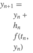 |
| 2 | Explicit Midpoint | 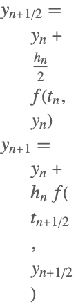 |
| 1 | Backward or Implicit Euler (1-stage RadauIIA) | 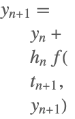 |
| 2 | Implicit Midpoint (1-stage Gauss) | 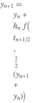 |
| 2 | Trapezoidal (2-stage Lobatto IIIA) | 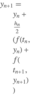 |
| 1 | Linearly Implicit Euler | 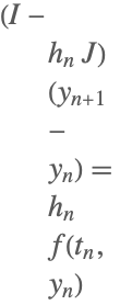 |
| 2 | Linearly Implicit Midpoint | 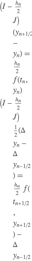 |
Some of the one-step methods that have been implemented.
Here ![]() ,
, ![]() denotes the identity matrix, and
denotes the identity matrix, and ![]() denotes the Jacobian matrix
denotes the Jacobian matrix ![]() .
.
Although the implicit midpoint method has not been implemented as a separate method, it is available through the one-stage Gauss scheme of the "ImplicitRungeKutta" method.