"SymplecticPartitionedRungeKutta" Method for NDSolve
| Introduction | Available Methods |
| Hamiltonian Systems | Automatic Order Selection |
| Rounding Error Reduction | Option Summary |
| Examples |
Introduction
When numerically solving Hamiltonian dynamical systems it is advantageous if the numerical method yields a symplectic map.
- The phase space of a Hamiltonian system is a symplectic manifold on which there exists a natural symplectic structure in the canonically conjugate coordinates.
- The time evolution of a Hamiltonian system is such that the Poincaré integral invariants associated with the symplectic structure are preserved.
- A symplectic integrator computes exactly, assuming infinite precision arithmetic, the evolution of a nearby Hamiltonian, whose phase space structure is close to that of the original system.
If the Hamiltonian can be written in separable form, ![]() , there exists an efficient class of explicit symplectic numerical integration methods.
, there exists an efficient class of explicit symplectic numerical integration methods.
An important property of symplectic numerical methods when applied to Hamiltonian systems is that a nearby Hamiltonian is approximately conserved for exponentially long times (see [BG94], [HL97], and [R99]).
Hamiltonian Systems
Consider a differential equation
A ![]() -degree of freedom Hamiltonian system is a particular instance of (1) with
-degree of freedom Hamiltonian system is a particular instance of (1) with ![]() , where
, where
Here ![]() represents the gradient operator:
represents the gradient operator:
and ![]() is the skew symmetric matrix:
is the skew symmetric matrix:
where ![]() and
and ![]() are the identity and zero
are the identity and zero ![]() ×
×![]() matrices.
matrices.
The components of ![]() are often referred to as position or coordinate variables and the components of
are often referred to as position or coordinate variables and the components of ![]() as the momenta.
as the momenta.
If ![]() is autonomous,
is autonomous, ![]() . Then
. Then ![]() is a conserved quantity that remains constant along solutions of the system. In applications, this usually corresponds to conservation of energy.
is a conserved quantity that remains constant along solutions of the system. In applications, this usually corresponds to conservation of energy.
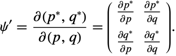
A numerical method applied to a Hamiltonian system (2) is said to be symplectic if it produces a symplectic map. That is, let ![]() be a
be a ![]() transformation defined in a domain
transformation defined in a domain ![]() :
:
where the Jacobian of the transformation is:
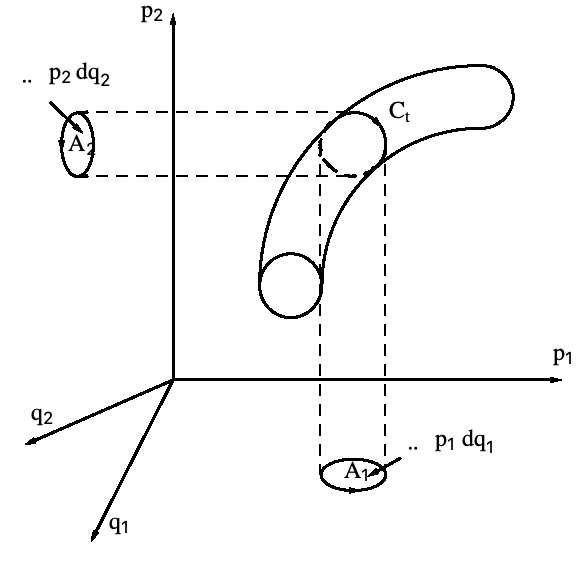
The flow of a Hamiltonian system is depicted together with the projection onto the planes formed by canonically conjugate coordinate and momenta pairs. The sum of the oriented areas remains constant as the flow evolves in time.
Partitioned Runge–Kutta Methods
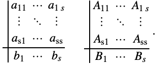
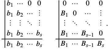
It is sometimes possible to integrate certain components of (3) using one Runge–Kutta method and other components using a different Runge–Kutta method. The overall ![]() -stage scheme is called a partitioned Runge–Kutta method and the free parameters are represented by two Butcher tableaux:
-stage scheme is called a partitioned Runge–Kutta method and the free parameters are represented by two Butcher tableaux:
Symplectic Partitioned Runge–Kutta (SPRK) Methods
For general Hamiltonian systems, symplectic Runge–Kutta methods are necessarily implicit.
However, for separable Hamiltonians ![]() there exist explicit schemes corresponding to symplectic partitioned Runge–Kutta methods.
there exist explicit schemes corresponding to symplectic partitioned Runge–Kutta methods.
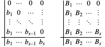
Instead of (4) the free parameters now take either the form:
The ![]() free parameters of (5) are sometimes represented using the shorthand notation
free parameters of (5) are sometimes represented using the shorthand notation ![]() .
.
The differential system for a separable Hamiltonian system can be written as:
In general the force evaluations ![]() are computationally dominant and (6) is preferred over (7) since it is possible to save one force evaluation per time step when dense output is required.
are computationally dominant and (6) is preferred over (7) since it is possible to save one force evaluation per time step when dense output is required.
Standard Algorithm
The structure of (8) permits a particularly simple implementation (see for example [SC94]).
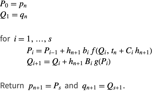
The time-weights are given by: ![]() .
.
If ![]() then Algorithm 1 effectively reduces to an
then Algorithm 1 effectively reduces to an ![]() stage scheme since it has the First Same As Last (FSAL) property.
stage scheme since it has the First Same As Last (FSAL) property.
Example
Needs["DifferentialEquations`NDSolveProblems`"];
Needs["DifferentialEquations`NDSolveUtilities`"];
The Harmonic Oscillator
The Harmonic oscillator is a simple Hamiltonian problem that models a material point attached to a spring. For simplicity consider the unit mass and spring constant for which the Hamiltonian is given in separable form:
The equations of motion are given by:
Input
system = GetNDSolveProblem["HarmonicOscillator"];
eqs = {system["System"], system["InitialConditions"]};
vars = system["DependentVariables"];
H = system["Invariants"];
time = {T, 0, 100};
step = 1 / 25;
Explicit Euler Method
solee = NDSolve[eqs, vars, time, Method -> "ExplicitEuler", StartingStepSize -> step, MaxSteps -> Infinity];ParametricPlot[Evaluate[vars /. First[solee]], Evaluate[time], PlotPoints -> 100]InvariantErrorPlot[H, vars, T, solee, PlotStyle -> Green]Symplectic Method
sol = NDSolve[eqs, vars, time, Method -> {"SymplecticPartitionedRungeKutta", "DifferenceOrder" -> 2, "PositionVariables" -> {Subscript[Y, 1][T]}}, StartingStepSize -> step, MaxSteps -> Infinity];ParametricPlot[Evaluate[vars /. First[sol]], Evaluate[time]]InvariantErrorPlot[H, vars, T, sol, PlotStyle -> Blue]Rounding Error Reduction
In certain cases, lattice symplectic methods exist and can avoid step-by-step roundoff accumulation, but such an approach is not always possible [ET92].
solnoca = NDSolve[eqs, vars, time, Method -> {"SymplecticPartitionedRungeKutta", "DifferenceOrder" -> 10, "PositionVariables" -> {Subscript[Y, 1][T]}}, StartingStepSize -> step, MaxSteps -> Infinity, "CompensatedSummation" -> False];


InvariantErrorPlot[H, vars, T, solnoca, PlotStyle -> Blue]
There is a curious drift in the error in the Hamiltonian that is actually a numerical artifact of floating-point arithmetic.
This phenomenon can have an impact on long time integrations.
This section describes the formulation used by "SymplecticPartitionedRungeKutta" in order to reduce the effect of such errors.
There are two types of errors in integrating a flow numerically, those along the flow and those transverse to the flow. In contrast to dissipative systems, the rounding errors in Hamiltonian systems that are transverse to the flow are not damped asymptotically.
Many numerical methods for ordinary differential equations involve computations of the form
where the increments ![]() are usually smaller in magnitude than the approximations
are usually smaller in magnitude than the approximations ![]() .
.
Let ![]() denote the exponent and
denote the exponent and ![]() ,
, ![]() , the mantissa of a number
, the mantissa of a number ![]() in precision
in precision ![]() radix
radix ![]() arithmetic:
arithmetic: ![]() .
.
Aligning according to exponents these quantities can be represented pictorially as
where numbers on the left have a smaller scale than numbers on the right.
Of interest is an efficient way of computing the quantities ![]() that effectively represent the radix
that effectively represent the radix ![]() digits discarded due to the difference in the exponents of
digits discarded due to the difference in the exponents of ![]() and
and ![]() .
.
Compensated Summation
The basic motivation for compensated summation is to simulate ![]() bit addition using only
bit addition using only ![]() bit arithmetic.
bit arithmetic.
Example
reps = 10^6;
base = 0.;
inc = 0.1;
Do[base = base + inc, {reps}];
InputForm[base]
In many applications the increment may vary and the number of operations is not known in advance.
Algorithm
Compensated summation (see for example [B87] and [H96]) computes the rounding error along with the sum so that
Algorithm 2 (Compensated Summation)
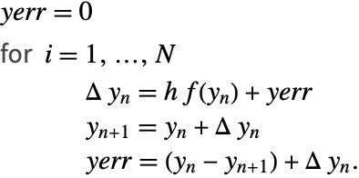
The algorithm is carried out componentwise for vectors.
Example
The function CompensatedPlus (in the Developer` context) implements the algorithm for compensated summation.
err = 0.;
base = 0.;
inc = 0.1;
Do[
	{base, err} =
	Developer`CompensatedPlus[base , inc, err],
	{reps}];
InputForm[base]
An undocumented option CompensatedSummation controls whether built-in integration methods in NDSolve use compensated summation.
An Alternative Algorithm
There are various ways that compensated summation can be used.
One way is to compute the error in every addition update in the main loop in Algorithm 1.
An alternative algorithm, which was proposed because of its more general applicability, together with reduced arithmetic cost, is given next. The essential ingredients are the increments ![]() and
and ![]() .
.
The desired values ![]() and
and ![]() are obtained using compensated summation.
are obtained using compensated summation.
Compensated summation could also be used in every addition update in the main loop of Algorithm 3, but our experiments have shown that this adds a non-negligible overhead for a relatively small gain in accuracy.
Numerical Illustration
Rounding Error Model
The amount of expected roundoff error in the relative error of the Hamiltonian for the harmonic oscillator (9) will now be quantified. A probabilistic average case analysis is considered in preference to a worst case upper bound.
For a one-dimensional random walk with equal probability of a deviation, the expected absolute distance after ![]() steps is
steps is ![]() .
.
The relative error for a floating-point operation ![]() ,
, ![]() ,
, ![]() ,
, ![]() using IEEE round to nearest mode satisfies the following bound [K93]:
using IEEE round to nearest mode satisfies the following bound [K93]:
where the base ![]() is used for representing floating-point numbers on the machine and
is used for representing floating-point numbers on the machine and ![]() for IEEE double-precision.
for IEEE double-precision.
Therefore the roundoff error after ![]() steps is expected to be approximately
steps is expected to be approximately
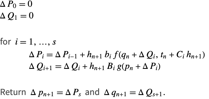
In the examples that follow a constant step size of 1/25 is used and the integration is performed over the interval [0, 80000] for a total of ![]() integration steps. The error in the Hamiltonian is sampled every 200 integration steps.
integration steps. The error in the Hamiltonian is sampled every 200 integration steps.
The 8 th-order 15-stage (FSAL) method D of Yoshida is used. Similar results have been obtained for the 6 th-order 7-stage (FSAL) method A of Yoshida with the same number of integration steps and a step size of 1/160.
Without Compensated Summation
The relative error in the Hamiltonian is displayed here for the standard formulation in Algorithm 1 (green) and for the increment formulation in Algorithm 3 (red) for the Harmonic oscillator (10).
Algorithm 1 for a 15-stage method corresponds to ![]() .
.
In the incremental Algorithm 3 the internal stages are all of the order of the step size and the only significant rounding error occurs at the end of each integration step; thus ![]() , which is in good agreement with the observed improvement.
, which is in good agreement with the observed improvement.
This shows that for Algorithm 3, with sufficiently small step sizes, the rounding error growth is independent of the number of stages of the method, which is particularly advantageous for high order.
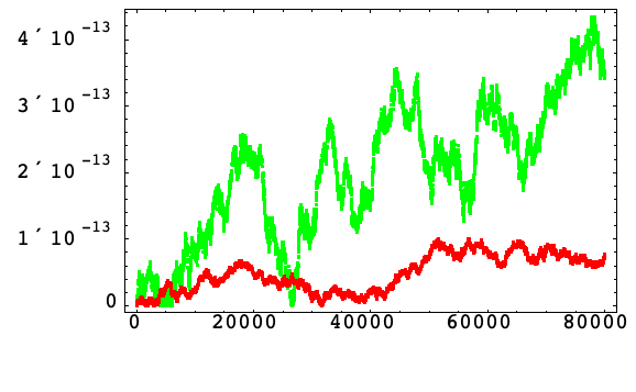
With Compensated Summation
The relative error in the Hamiltonian is displayed here for the increment formulation in Algorithm 3 without compensated summation (red) and with compensated summation (blue) for the Harmonic oscillator (11).
Using compensated summation with Algorithm 3, the error growth appears to satisfy a random walk with deviation ![]() so that it has been reduced by a factor proportional to the step size.
so that it has been reduced by a factor proportional to the step size.
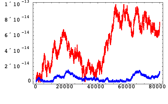
Arbitrary Precision
The relative error in the Hamiltonian is displayed here for the increment formulation in Algorithm 3 with compensated summation using IEEE double-precision arithmetic (blue) and with 32-decimal-digit software arithmetic (purple) for the Harmonic oscillator (12).
However, the solution obtained using software arithmetic is around an order of magnitude slower than machine arithmetic, so strategies to reduce the effect of roundoff error are worthwhile.
Examples
Electrostatic Wave
Here is a non-autonomous Hamiltonian (it has a time-dependent potential) that models ![]() perturbing electrostatic waves, each with the same wave number and amplitude, but different temporal frequencies
perturbing electrostatic waves, each with the same wave number and amplitude, but different temporal frequencies ![]() (see [CR91]).
(see [CR91]).
H = p[t] ^ 2 / 2 + q[t] ^ 2 / 2 + Sum[Cos[q[t] - 7 i t], {i, 3}];
eqs = {p'[t]  == -D[H, q[t]], q'[t] == D[H, p[t]]};
ics = {p[0] == 0, q[0] == 4483 / 400};
vars = {q[t], p[t]};
time = {t, 0, 10000 2 π};
step = 2 π / 105;
A general technique for computing Poincaré sections is described within "Events and Discontinuities in Differential Equations". Specifying an empty list for the variables avoids storing all the data of the numerical integration.
sprkmethod = {"SymplecticPartitionedRungeKutta", "DifferenceOrder" -> 4, "PositionVariables" -> {q[t]}};


sprkdata =
	Block[{k = 1},
	Reap[
	NDSolve[{eqs, ics, WhenEvent[Mod[t, 2 Pi] == 0, Sow[{q[t], p[t]}]]}, {}, time, Method -> sprkmethod, StartingStepSize -> step, MaxSteps -> Infinity
	];
	]
];ListPlot[sprkdata[[-1, 1]], Axes -> False, Frame -> True, AspectRatio -> 1, PlotRange -> All]rkmethod = {"FixedStep", Method -> {"ExplicitRungeKutta", "DifferenceOrder" -> 4}};
rkdata =
Block[{k = 1},
Reap[
NDSolve[{eqs, ics, WhenEvent[Mod[t, 2 Pi] == 0, Sow[{q[t], p[t]}]]}, {}, time, Method -> rkmethod, StartingStepSize -> step, MaxSteps -> Infinity
];
]
];ListPlot[rkdata[[-1, 1]], Axes -> False, Frame -> True, AspectRatio -> 1, PlotRange -> All]Toda Lattice
The Toda lattice models particles on a line interacting with pairwise exponential forces and is governed by the Hamiltonian:
Consider the case when periodic boundary conditions ![]() are enforced.
are enforced.
The Toda lattice is an example of an isospectral flow. Using the notation
then the eigenvalues of the following matrix are conserved quantities of the flow:
n = 3;
periodicRule = {Subscript[q, n + 1][t] -> Subscript[q, 1][t]};
H = Underoverscript[∑, k = 1, n]((Subscript[p, k][t]^2/2) + (Exp[Subscript[q, k + 1][t] - Subscript[q, k][t]] - 1)) /. periodicRule;
eigenvalueRule = {Subscript[a, k_][t] :> -Subscript[p, k][t] / 2, Subscript[b, k_][t] :> 1 / 2Exp[1 / 2(Subscript[q, k + 1][t] - Subscript[q, k][t])]};
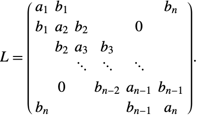
L = (| | | |
| ----- | ----- | ----- |
| a1[t] | b1[t] | b3[t] |
| b1[t] | a2[t] | b2[t] |
| b3[t] | b2[t] | a3[t] |) /. eigenvalueRule /. periodicRule;
eqs = {Subscript[q, 1]'[t] == D[H, Subscript[p, 1][t]], Subscript[q, 2]'[t] == D[H, Subscript[p, 2][t]], Subscript[q, 3]'[t] == D[H, Subscript[p, 3][t]], Subscript[p, 1]'[t] == -D[H, Subscript[q, 1][t]], Subscript[p, 2]'[t] == -D[H, Subscript[q, 2][t]], Subscript[p, 3]'[t] == -D[H, Subscript[q, 3][t]]};
ics = {Subscript[q, 1][0] == 1, Subscript[q, 2][0] == 2, Subscript[q, 3][0] == 4, Subscript[p, 1][0] == 0, Subscript[p, 2][0] == 1, Subscript[p, 3][0] == 1 / 2};
eqs = {eqs, ics};
vars = {Subscript[q, 1][t], Subscript[q, 2][t], Subscript[q, 3][t], Subscript[p, 1][t], Subscript[p, 2][t], Subscript[p, 3][t]};
time = {t, 0, 50};NumberMatrixQ[m_] := MatrixQ[m, NumberQ];
NumberEigenvalues[m_ ? NumberMatrixQ] := Sort[Eigenvalues[m]];emsol = NDSolve[eqs, vars, time, Method -> "ExplicitMidpoint", StartingStepSize -> 1 / 10];The absolute error in the eigenvalues is now plotted throughout the integration interval.
Options are used to specify the dimension of the result of NumberEigenvalues (since it is not an explicit list) and that the absolute error specified using InvariantErrorFunction should include the sign of the error (the default uses Abs).
InvariantErrorPlot[NumberEigenvalues[L], vars, t, emsol, InvariantErrorFunction -> (#1 - #2&),
InvariantDimensions -> {n}, PlotStyle -> {Red, Blue, Green}]sprksol = NDSolve[eqs, vars, time, Method -> {"SymplecticPartitionedRungeKutta", DifferenceOrder -> 2, "PositionVariables" -> {Subscript[q, 1][t], Subscript[q, 2][t], Subscript[q, 3][t]}}, StartingStepSize -> 1 / 10];InvariantErrorPlot[NumberEigenvalues[L], vars, t, sprksol, InvariantErrorFunction -> (#1 - #2&),
InvariantDimensions -> {n}, PlotStyle -> {Red, Blue, Green}]Some recent work on numerical methods for isospectral flows can be found in [CIZ97], [CIZ99], [DLP98a], and [DLP98b].
Available Methods
Default Methods
The following table lists the current default choice of SPRK methods.
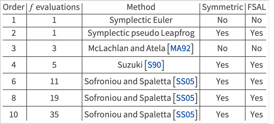
Unlike the situation for explicit Runge–Kutta methods, the coefficients for high-order SPRK methods are only given numerically in the literature. Yoshida [Y90] only gives coefficients accurate to 14 decimal digits of accuracy for example.
Since NDSolve also works for arbitrary precision, you need a process for obtaining the coefficients to the same precision as that to be used in the solver.
When the closed form of the coefficients is not available, the order equations for the symmetric composition coefficients can be refined in arbitrary precision using FindRoot, starting from the known machine-precision solution.
Alternative Methods
Due to the modular design of the new NDSolve framework it is straightforward to add an alternative method and use that instead of one of the default methods.
Several checks are made before any integration is carried out:
- The two vectors of coefficients should be nonempty, the same length, and numerical approximations should yield number entries of the correct precision.
Example
system = GetNDSolveProblem["PerturbedKepler"];
time = {T, 0, 290};
step = 1 / 25;YoshidaCoefficients[4, prec_] :=
N[
{{Root[-1 + 12 * #1 - 48 * #1 ^ 2 + 48 * #1 ^ 3&, 1, 0], Root[1 - 24 * #1 ^ 2 + 48 * #1 ^ 3&, 1, 0], Root[1 - 24 * #1 ^ 2 + 48 * #1 ^ 3&, 1, 0], Root[-1 + 12 * #1 - 48 * #1 ^ 2 + 48 * #1 ^ 3&, 1, 0]}, {Root[-1 + 6 * #1 - 12 * #1 ^ 2 + 6 * #1 ^ 3&, 1, 0], Root[1 - 3 * #1 + 3 * #1 ^ 2 + 3 * #1 ^ 3&, 1, 0], Root[-1 + 6 * #1 - 12 * #1 ^ 2 + 6 * #1 ^ 3&, 1, 0], 0}},
prec];YoshidaCoefficients[4, MachinePrecision]Yoshida4 = {"SymplecticPartitionedRungeKutta", "Coefficients" -> YoshidaCoefficients, "DifferenceOrder" -> 4, "PositionVariables" -> {Subscript[Y, 1][T], Subscript[Y, 2][T]}};
Yoshida4sol = NDSolve[system, time, Method -> Yoshida4, StartingStepSize -> step, MaxSteps -> Infinity];ParametricPlot[Evaluate[{Subscript[Y, 1][T], Subscript[Y, 2][T]} /. Yoshida4sol], Evaluate[time]]Automatic Order Selection
Given that a variety of methods of different orders are available, it is useful to have a means of automatically selecting an appropriate method. In order to accomplish this we need a measure of work for each method.
A reasonable measure of work for an SPRK method is the number of stages ![]() (or
(or ![]() if the method is FSAL).
if the method is FSAL).
Definition (Work per unit step)
Given a step size ![]() and a work estimate
and a work estimate ![]() for one integration step with a method of order
for one integration step with a method of order ![]() , the work per unit step is given by
, the work per unit step is given by ![]() .
.
Let ![]() be a nonempty set of method orders,
be a nonempty set of method orders, ![]() denote the
denote the ![]() th element of
th element of ![]() , and
, and ![]() denote the cardinality (number of elements).
denote the cardinality (number of elements).
A comparison of work for the default SPRK methods gives ![]() .
.
A prerequisite is a procedure for estimating the starting step ![]() of a numerical method of order
of a numerical method of order ![]() (see for example [GSB87] or [HNW93]).
(see for example [GSB87] or [HNW93]).
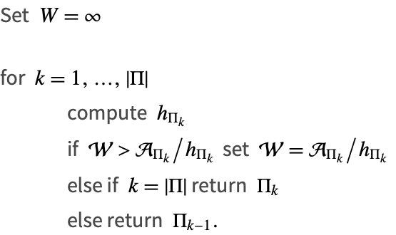
The first case to be considered is when the starting step estimate ![]() can be freely chosen. By bootstrapping from low order, the following algorithm finds the order that locally minimizes the work per unit step.
can be freely chosen. By bootstrapping from low order, the following algorithm finds the order that locally minimizes the work per unit step.
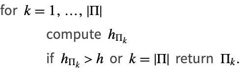
The second case to be considered is when the starting step estimate h is given. The following algorithm then gives the order of the method that minimizes the computational cost while satisfying given absolute and relative local error tolerances.
Algorithms 4 and 5 are heuristic since the optimal step size and order may change through the integration, although symplectic integration often involves fixed choices. Despite this, both algorithms incorporate salient integration information, such as local error tolerances, system dimension, and initial conditions, to avoid poor choices.
Examples
Consider Kepler's problem that describes the motion in the configuration plane of a material point that is attracted toward the origin with a force inversely proportional to the square of the distance:
Algorithm 4
The following figure shows the methods chosen automatically at various tolerances for the Kepler problem (14) according to Algorithm 4 on a log-log scale of maximum absolute phase error versus work.
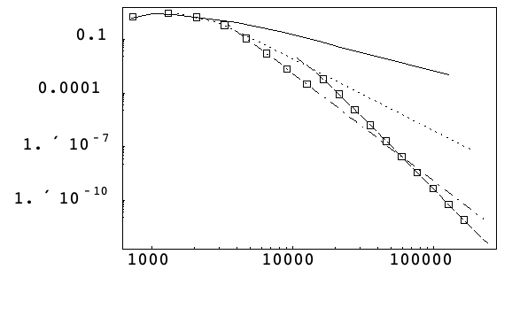
It can be observed that the algorithm does a reasonable job of staying near the optimal method, although it switches over to the 8 th-order method slightly earlier than necessary.
This can be explained by the fact that the starting step size routine is based on low-order derivative estimation and this may not be ideal for selecting high-order methods.
Algorithm 5
The following figure shows the methods chosen automatically with absolute local error tolerance of 10-9 and step sizes 1/16, 1/32, 1/64, 1/128 for the Kepler problem (15) according to Algorithm 5 on a log-log scale of maximum absolute phase error versus work.
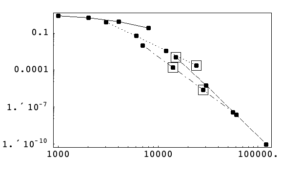
With the local tolerance and step size fixed the code can only choose the order of the method.
For large step sizes a high-order method is selected, whereas for small step sizes a low-order method is selected. In each case the method chosen minimizes the work to achieve the given tolerance.
Option Summary
option name | default value | |
| "Coefficients" | "SymplecticPartitionedRungeKuttaCoefficients" | specify the coefficients of the symplectic partitioned Runge–Kutta method |
| "DifferenceOrder" | Automatic | specify the order of local accuracy of the method |
| "PositionVariables" | {} | specify a list of the position variables in the Hamiltonian formulation |