"Composition" and "Splitting" Methods for NDSolve
Introduction
In some cases it is useful to split the differential system into subsystems and solve each subsystem using appropriate integration methods. Recombining the individual solutions often allows certain dynamical properties, such as volume, to be conserved. More information on splitting and composition can be found in [MQ02, HLW02], and specific aspects related to NDSolve are discussed in [SS05, SS06].
Definitions
Of concern are initial value problems ![]() , where
, where ![]() .
.
"Composition"
Composition is a useful device for raising the order of a numerical integration scheme.
In contrast to the Aitken–Neville algorithm used in extrapolation, composition can conserve geometric properties of the base integration method (e.g. symplecticity).
Let ![]() be a basic integration method that takes a step of size
be a basic integration method that takes a step of size ![]() with
with ![]() given real numbers.
given real numbers.
Then the ![]() -stage composition method
-stage composition method ![]() is given by
is given by
Often interest is in composition methods ![]() that involve the same base method
that involve the same base method ![]()
An interesting special case is symmetric composition: ![]() ,
, ![]() .
.
The most common types of composition are:
"Splitting"
An ![]() -stage splitting method is a generalization of a composition method in which
-stage splitting method is a generalization of a composition method in which ![]() is broken up in an additive fashion:
is broken up in an additive fashion:
The essential point is that there can often be computational advantages in solving problems involving ![]() instead of
instead of ![]() .
.
An ![]() -stage splitting method is a composition of the form
-stage splitting method is a composition of the form
with ![]() not necessarily distinct.
not necessarily distinct.
Each base integration method now only solves part of the problem, but a suitable composition can still give rise to a numerical scheme with advantageous properties.
If the vector field ![]() is integrable, then the exact solution or flow
is integrable, then the exact solution or flow ![]() can be used in place of a numerical integration method.
can be used in place of a numerical integration method.
A splitting method may also use a mixture of flows and numerical methods.
An example is Lie–Trotter splitting [T59]:
Split ![]() with
with ![]() ; then
; then ![]() yields a first-order integration method.
yields a first-order integration method.
Computationally it can be advantageous to combine flows using the group property
Implementation
Several changes to the new NDSolve framework were needed in order to implement splitting and composition methods.
- Add the ability to pass around a function for numerically evaluating a subfield, instead of the entire vector field.
- Add a "LocallyExact" method to compute the flow; analytically solve a subsystem and advance the (local) solution numerically.
- Add cache data for identical methods to avoid repeated initialization. Data for numerically evaluating identical subfields is also cached.
A simplified input syntax allows omitted vector fields and methods to be filled in cyclically. These must be defined unambiguously:
Nested Methods
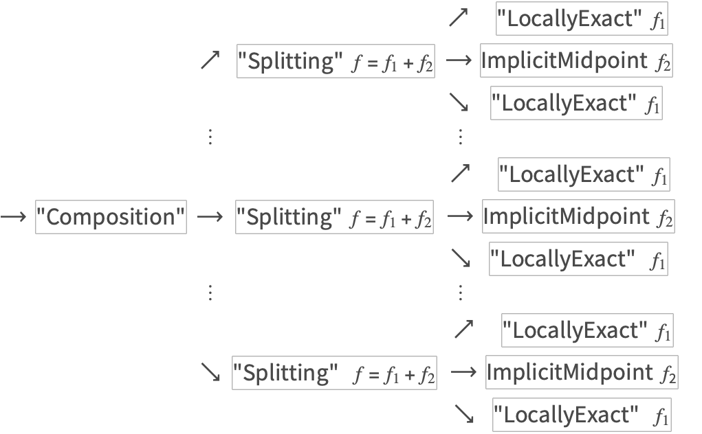
The following example constructs a high-order splitting method from a low-order splitting using "Composition".
Simplification
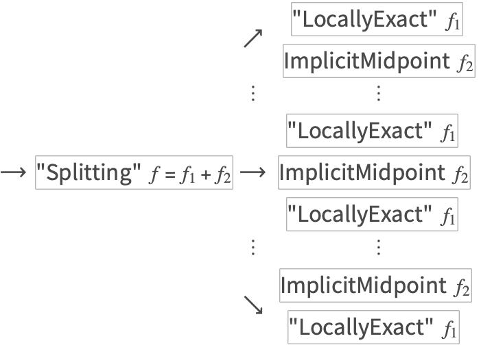
A more efficient integrator can be obtained in the previous example using the group property of flows and calling the "Splitting" method directly.
Examples
The following examples will use a second-order symmetric splitting known as the Strang splitting [S68], [M68]. The splitting coefficients are automatically determined from the structure of the equations.
Symplectic Splitting
Symplectic Leapfrog
"SymplecticPartitionedRungeKutta" is an efficient method for solving separable Hamiltonian systems ![]() with favorable long-time dynamics.
with favorable long-time dynamics.
"Splitting" is a more general-purpose method, but it can be used to construct partitioned symplectic methods (though it is somewhat less efficient than "SymplecticPartitionedRungeKutta").
The method "ExplicitEuler" could only have been specified once, since the second and third instances would have been filled in cyclically.
Composition of Symplectic Leapfrog
Hybrid Methods
While a closed-form solution often does not exist for the entire vector field, in some cases it is possible to analytically solve a system of differential equations for part of the vector field.
When a solution can be found by DSolve, direct numerical evaluation can be used to locally advance the solution.
This idea is implemented in the method "LocallyExact".
Harmonic Oscillator Test Example
Hybrid Numeric-Symbolic Splitting Methods (ABC Flow)
When applied directly, a volume-preserving integrator would not in general preserve symmetries. A symmetry-preserving integrator, such as the implicit midpoint rule, would not preserve volume.
The system for Y2 is solvable exactly by DSolve so that you can use the "LocallyExact" method.
Y1 is not solvable, however, so you need to use a suitable numerical integrator in order to obtain the desired properties in the splitting method.
Lotka–Volterra Equations
Various numerical integrators for this system are compared within "Numerical Methods for Solving the Lotka–Volterra Equations".
Euler's Equations
Various numerical integrators for Euler's equations are compared within "Rigid Body Solvers".
Non-Autonomous Vector Fields
Option Summary
The default coefficient choice in "Composition" tries to automatically select between "SymmetricCompositionCoefficients" and "SymmetricCompositionSymmetricMethodCoefficients" depending on the properties of the methods specified using the Method option.
option name | default value | |
| "Coefficients" | Automatic | specify the coefficients to use in the composition method |
| "DifferenceOrder" | Automatic | specify the order of local accuracy of the method |
| Method | None | specify the base methods to use in the numerical integration |
Options of the method "Composition".
option name | default value | |
| "Coefficients" | {} | specify the coefficients to use in the splitting method |
| "DifferenceOrder" | Automatic | specify the order of local accuracy of the method |
| "Equations" | {} | specify the way in which the equations should be split |
| Method | None | specify the base methods to use in the numerical integration |