
10.2 Three-Dimensional Graphics Directives
In three dimensions, just as in two dimensions, you can give various graphics directives to specify how the different elements in a graphics object should be rendered.
All the graphics directives for two dimensions also work in three dimensions. There are however some additional directives in three dimensions.
Just as in two dimensions, you can use the directives PointSize, Thickness and Dashing to tell Mathematica TE how to render Point and Line elements. Note that in three dimensions, the lengths that appear in these directives are measured as fractions of the total width of the display area for your plot.
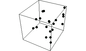
This generates a list of 20 random points in three dimensions.
In[1]:= pts = Table[Point[Table[Random[ ], {3}]], {20}];
This displays the points, with each one being a circle whose diameter is 5% of the display area width.
In[2]:= Show[Graphics3D[ { PointSize[0.05], pts } ]]
Out[2]= 
As in two dimensions, you can use AbsolutePointSize, AbsoluteThickness and AbsoluteDashing if you want to measure length in absolute units.
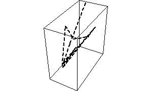
This generates a line through 10 random points in three dimensions.
In[3]:= line = Line[Table[Random[ ], {10}, {3}]] ;
This shows the line dashed, with a thickness of 2 printer's points.
In[4]:= Show[Graphics3D[ { AbsoluteThickness[2],
AbsoluteDashing[{5, 5}], line } ]]
Out[4]= 
For Point and Line objects, the color specification directives also work the same in three dimensions as in two dimensions. For Polygon objects, however, they can work differently.
In two dimensions, polygons are always assumed to have an intrinsic color, specified directly by graphics directives such as RGBColor. In three dimensions, however, Mathematica TE also provides the option of generating colors for polygons using a more physical approach based on simulated illumination. With the default option setting Lighting -> True for Graphics3D objects, Mathematica TE ignores explicit colors specified for polygons, and instead determines all polygon colors using the simulated illumination model. Even in this case, however, explicit colors are used for points and lines.

The two schemes for coloring polygons in three dimensions.
This loads a package that defines various polyhedra.
In[5]:= <<Graphics`Polyhedra` ;
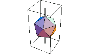
This draws an icosahedron, using the same gray level for all faces.
In[6]:= Show[Graphics3D[{GrayLevel[0.7], Icosahedron[ ]}],
Lighting -> False]
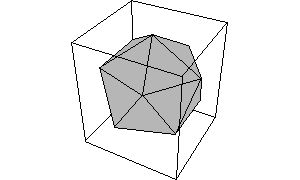
Out[6]= 
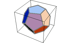
With the default setting Lighting -> True, the colors of polygons are determined by the simulated illumination model, and explicit color specifications are ignored.
In[7]:= Show[%, Lighting -> True]
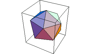
Out[7]= 
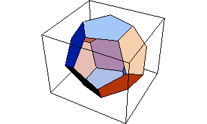
Explicit color directives are, however, always followed for points and lines.
In[8]:= Show[{%, Graphics3D[{GrayLevel[0.5], Thickness[0.05],
Line[{{0, 0, -2}, {0, 0, 2}}]}]}]
Out[8]= 

Giving graphics directives for the edges of polygons.
When you render a three-dimensional graphics object in Mathematica TE, there are two kinds of lines that can appear. The first kind are lines from explicit Line primitives that you included in the graphics object. The second kind are lines that were generated as the edges of polygons.
You can tell Mathematica TE how to render lines of the second kind by giving a list of graphics directives inside EdgeForm.
This renders a dodecahedron with its edges shown as thick gray lines.
In[9]:= Show[Graphics3D[
{EdgeForm[{GrayLevel[0.5], Thickness[0.02]}],
Dodecahedron[ ]}]]
Out[9]= 

Rendering the fronts and backs of polygons differently.
An important aspect of polygons in three dimensions is that they have both front and back faces. Mathematica TE uses the following convention to define the "front face" of a polygon: if you look at a polygon from the front, then the corners of the polygon will appear counterclockwise, when taken in the order that you specified them.
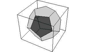
This defines a dodecahedron with one face removed.
In[10]:= d = Drop[Dodecahedron[ ], {6}] ;
You can now see inside the dodecahedron.
In[11]:= Show[Graphics3D[d]]
Out[11]= 
This makes the front (outside) face of each polygon light gray, and the back (inside) face dark gray.
In[12]:= Show[Graphics3D[{FaceForm[GrayLevel[0.8], GrayLevel[0.3]], d}], Lighting -> False]
Out[12]= 