15.5 The Uncertainties of Numerical Mathematics
Mathematica TE does operations like numerical integration very differently from the way it does its symbolic counterparts.
When you do a symbolic integral, Mathematica TE takes the functional form of the integrand you have given, and applies a sequence of exact symbolic transformation rules to it, to try and evaluate the integral.
When you do a numerical integral, however, Mathematica TE does not look directly at the functional form of the integrand you have given. Instead, it simply finds a sequence of numerical values of the integrand at particular points, then takes these values and tries to deduce from them a good approximation to the integral.
An important point to realize is that when Mathematica TE does a numerical integral, the only information it has about your integrand is a sequence of numerical values for it. To get a definite result for the integral, Mathematica TE then effectively has to make certain assumptions about the smoothness and other properties of your integrand. If you give a sufficiently pathological integrand, these assumptions may not be valid, and as a result, Mathematica TE may simply give you the wrong answer for the integral.
This problem may occur, for example, if you try to integrate numerically a function that has a very thin spike at a particular position. Mathematica TE samples your function at a number of points, and then assumes that the function varies smoothly between these points. As a result, if none of the sample points come close to the spike, then the spike will go undetected, and its contribution to the numerical integral will not be correctly included.
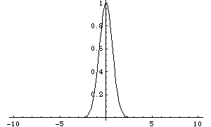
Here is a plot of the function  .
.
In[1]:= Plot[Exp[-x^2], {x, -10, 10}, PlotRange->All]

Out[1]= 
NIntegrate gives the correct answer for the numerical integral of this function from  to
to  .
.
In[2]:= NIntegrate[Exp[-x^2], {x, -10, 10}]
Out[2]= 
If, however, you ask for the integral from  to
to  , NIntegrate will miss the peak near
  , and give the wrong answer.
In[3]:= NIntegrate[Exp[-x^2], {x, -1000, 1000}]

Out[3]= 
Although NIntegrate follows the principle of looking only at the numerical values of your integrand, it nevertheless tries to make the best possible use of the information that it can get. Thus, for example, if NIntegrate notices that the estimated error in the integral in a particular region is large, it will take more samples in that region. In this way, NIntegrate tries to "adapt" its operation to the particular integrand you have given.
The kind of adaptive procedure that NIntegrate uses is similar, at least in spirit, to what Plot does in trying to draw smooth curves for functions. In both cases, Mathematica TE tries to go on taking more samples in a particular region until it has effectively found a smooth approximation to the function in that region.
The kinds of problems that can appear in numerical integration can also arise when doing other numerical operations on functions.
For example, if you ask for a numerical approximation to the sum of an infinite series, Mathematica TE samples a certain number of terms in the series, and then does an extrapolation to estimate the contributions of other terms. If you insert large terms far out in the series, they may not be detected when the extrapolation is done, and the result you get for the sum may be incorrect.
A similar problem arises when you try to find a numerical approximation to the minimum of a function. Mathematica TE samples only a finite number of values, then effectively assumes that the actual function interpolates smoothly between these values. If in fact the function has a sharp dip in a particular region, then Mathematica TE may miss this dip, and you may get the wrong answer for the minimum.
If you work only with numerical values of functions, there is simply no way to avoid these kinds of problems. Exact symbolic computation, of course, allows you to get around these problems.
In many calculations, it is therefore worthwhile to go as far as you can symbolically, and then resort to numerical methods only at the very end. This gives you the best chance of avoiding the problems that can arise in purely numerical computations.
You might imagine that you could use symbolic methods to check for any features, say in the integrand of a numerical integral, that would give rise to problems in numerical computation. As soon as your integrand contains conditionals, control structures or nested function calls, there can be no general procedure, however, to do the tests that are needed. Nevertheless, for specific classes of integrands, it may be possible to perform some such tests. You can always implement these tests by defining special rules for NIntegrate in certain cases.