
9.2 Graphics Directives and Options
When you set up a graphics object in Mathematica TE, you typically give a list of graphical elements. You can include in that list graphics directives that specify how subsequent elements in the list should be rendered.
In general, the graphical elements in a particular graphics object can be given in a collection of nested lists. When you insert graphics directives in this kind of structure, the rule is that a particular graphics directive affects all subsequent elements of the list it is in, together with all elements of sublists that may occur. The graphics directive does not, however, have any effect outside the list it is in.
The first sublist contains the graphics directive GrayLevel.
In[1]:= {{GrayLevel[0.5], Rectangle[{0, 0}, {1, 1}]},
Rectangle[{1, 1}, {2, 2}]}
Out[1]= 
Only the rectangle in the first sublist is affected by the GrayLevel directive.
In[2]:= Show[Graphics[ % ]]

Out[2]= 
Mathematica TE provides various kinds of graphics directives. One important set is those for specifying the colors of graphical elements. Even if you have a black-and-white display device, you can still give color graphics directives. The colors you specify will be converted to gray levels at the last step in the graphics rendering process. Note that you can get black-and-white output even on a color device by setting the option ColorOutput -> GrayLevel.

Basic Mathematica color specifications.
On a color display, the two curves would be shown in color. Here they are shown in gray.
In[3]:= Plot[{x^2, x^3}, {x, 1, 3},
PlotStyle ->
{{RGBColor[1, 0, 0]}, {RGBColor[0, 1, 0]}}]
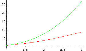
Out[3]= 
The function Hue[h] provides a convenient way to specify a range of colors using just one parameter. As h varies from 0 to 1, Hue[h] runs through red, yellow, green, cyan, blue, magenta, and back to red again. Hue[h, s, b] allows you to specify not only the "hue", but also the "saturation" and "brightness" of a color. Taking the saturation to be equal to one gives the deepest colors; decreasing the saturation towards zero leads to progressively more "washed out" colors.
For most purposes, you will be able to specify the colors you need simply by giving appropriate RGBColor or Hue directives.
When you give a graphics directive such as RGBColor, it affects all subsequent graphical elements that appear in a particular list. Mathematica TE also supports various graphics directives that affect only specific types of graphical elements.
The graphics directive PointSize[d] specifies that all Point elements, which appear in a graphics object, should be drawn as circles with a diameter d. In PointSize, the diameter d is measured as a fraction of the width of your whole plot.
Mathematica TE also provides the graphics directive AbsolutePointSize[d], which allows you to specify the "absolute" diameter of points, measured in fixed units. The units are approximately printer's points, equal to  of an inch.

Graphics directives for points.
Here is a list of points.
In[4]:= Table[Point[{n, Prime[n]}], {n, 6}]
Out[4]= 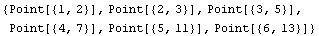
This makes each point have a diameter equal to one-tenth of the width of the plot.
In[5]:= Show[Graphics[{PointSize[0.1], %}], PlotRange -> All]

Out[5]= 
Here each point has size 3 in absolute units.
In[6]:= ListPlot[Table[Prime[n], {n, 20}],
Prolog -> AbsolutePointSize[3]]
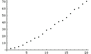
Out[6]= 

Graphics directives for lines.
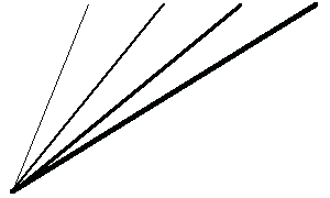
This generates a list of lines with different absolute thicknesses.
In[7]:= Table[
{AbsoluteThickness[n], Line[{{0, 0}, {n, 1}}]}, {n, 4}]
Out[7]= 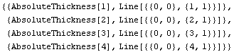
Here is a picture of the lines.
In[8]:= Show[Graphics[%]]
Out[8]= 
The Dashing graphics directive allows you to create lines with various kinds of dashing. The basic idea is to break lines into segments that are alternately drawn and omitted. By changing the lengths of the segments, you can get different line styles. Dashing allows you to specify a sequence of segment lengths. This sequence is repeated as many times as necessary in drawing the whole line.
This gives a dashed line and a dot-dashed line.
In[9]:= Show[Graphics[{
Dashing[{0.05, 0.05}],
Line[{{-1, -1}, {1, 1}}],
Dashing[{0.01, 0.05, 0.05, 0.05}],
Line[{{-1, 1}, {1, -1}}]
}]]
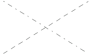
Out[9]= 