
Graphics
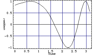
Here is a plot of the function  , with
  ranging from
  to
to  .
.
In[1]:= Plot[ Sin[ 2^x ], {x, 0, Pi} ]

Out[1]= 
Mathematica TE provides many options that you can set to determine exactly how your plots will look.
In[2]:= Show[ %, Frame -> True,
FrameLabel -> {"Time", "Signal"},
GridLines -> Automatic ]
Out[2]= 
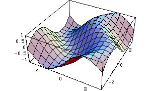
Here is a three-dimensional surface plot of a function of two variables.
In[3]:= Plot3D[ Sin[x + Sin[y]], {x, -3, 3}, {y, -3, 3} ]
Out[3]= 
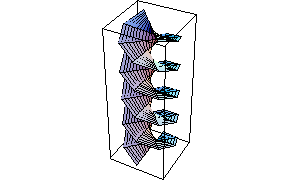
This generates a three-dimensional parametric surface. The  ,
,  and
and  coordinates of points on the surface are specified as a function of the parameters
  and
and  . The space in u Sin[t] denotes multiplication.
In[4]:= ParametricPlot3D[ {u Sin[t], u Cos[t], t/3},
{t, 0, 15}, {u, -1, 1}, Ticks -> None ]
Out[4]= 
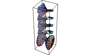
Here is a more complicated parametric surface.
In[5]:= ParametricPlot3D[
{Sin[t], Sin[2t] Sin[u], Sin[2t] Cos[u]},
{t, -Pi/2, Pi/2}, {u, 0, 2 Pi}, Ticks -> None ]

Out[5]= 
Mathematica TE allows you to combine different pieces of graphics together. The % stands for the last result; the %% for the result before that.
In[6]:= Show[%, %%]
Out[6]= 
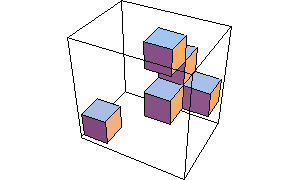
Mathematica TE serves as a graphics language in which you can build up graphics from components. In this case, a three-dimensional graphic is built up from a collection of cubes placed at different points.
In[7]:= Show[ Graphics3D[
{Cuboid[{0, 0, 0}], Cuboid[{2, 2, 2}],
Cuboid[{2, 1, 3}], Cuboid[{3, 2, 1}],
Cuboid[{2, 1, 1}]} ]]
Out[7]= 
On computer systems with sound output, this generates an 8-second long sound with the specified amplitude as a function of time.
In[8]:= Play[ Sin[10000 / t], {t, -4, 4} ]
Out[8]= -Sound-