Solids of Revolution - The Shell Method
I used the following notebook to demonstrate finding the volume of solids of revolution using approximating shells. After evaluating the first command in this notebook, you will be asked "Do you want to automatically evaluate all the initialization cells in the notebook?" Click Yes, and Mathematica will automatically evaluate the commands under "Initialization Code."
The most complicated part of these graphics is dealing with the many options involved: What are we rotating around? Do I want to look at the solid from the top, the bottom, the side, or somewhere else? This picture is too tall (or short)--how can I make it a more manageable size? To keep things from being too intimidating for my students, I set a bunch of defaults for the particular example I was doing in the initialization section.
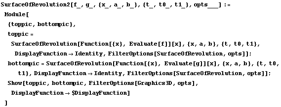
First, I made a picture of the solid generated by rotating the region between  and the x-axis around the y-axis. The code for SurfaceOfRevolution2 is in the initialization section, but it basically draws the two surfaces (one for each bounding curve) and combines them together in a single picture. I used two different viewpoints to help visualize the solid. I named the first picture pic1 so I could use it in a later example.

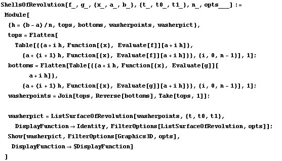
Here, the solid has been sliced into ten approximating shells.

In this picture, a single shell is shown along with a wireframe view of the original solid.

This is the same picture, but looking down along the axis of revolution.

The following table of graphics shows the visual effect of using more and more approximating shells. Mathematica will animate the graphics in a flip-book fashion when you double-click any of the graphics generated. The presentation is a bit tidier if you close the group of cells containing all the graphics using the brackets on the far right-hand side of the screen, but that is not necessary.
The animation reinforces the concept that as the number of subdivisions increases, the shells actually get closer and closer to the original solid.

In a second example, we considered rotating the region between  and
and  around the y-axis.

Since it is hard to see the inside of the bowl in this picture, I used an additional argument to SurfaceOfRevolution to cut a small slice out of the bowl. After the two functions and the domain, you can include an angle specification to tell Mathematica how much of the rotated figure you want. Here, I left a small gap between  radians and
  radians.

Here are approximations of the previous two figures using shells.

Initialization Code
These commands load the extra functions used in this notebook.

This sets the default axis of rotation to the y-axis. The x-axis would be {1,0}. Using AspectRatio 1 makes the pictures square so it is easier to see the whole picture at once.

Here is the code for the SurfaceOfRevolution2 and ShellsOfRevolution functions.


