10.1 Linear Quadratic Regulator

In the case of the linear system

or

and quadratic cost functions, the optimal control problem is said to be the linear-quadratic (LQ) optimal control problem. Further, for constant-coefficient matrices and and terminal time infinitely far in the future (meaning, of course, that the operating time is sufficiently long compared to the time constants of the system), the problem is referred to as the infinite-horizon or infinite-time-to-go problem. In this case, the control law in Eq. (10.3) simplifies to

with a constant-coefficient feedback gain matrix K. Note that the penalty function for terminal constraint in Eq. (10.2) and Eq. (10.8) is not an issue for the infinite-horizon problem. The function LQRegulatorGains attempts to find the matrix K for this particular case. It recognizes the type of system supplied to its input—continuous- versus discrete-time—and acts accordingly. As is the case with the pole assignment problem, furnishing matrices and in the state-space description is optional.

Linear quadratic regulator design.

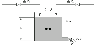
As an example, we design an optimal regulator for the mixing tank shown in Figure 10.1. The tank (Gopal (1993)) implements concentration control of a chemical mixture with inflows through two regulated valves at rates and and concentrations and , respectively. Outflow is at the rate with concentration . The volume of the liquid in the tank is . The state, input, and output vectors are assumed to be as follows:

The design will be carried out in the discrete-time domain.

Figure 10.1. Mixing tank schematic.

Load the application.

In[1]:=

This is a state-space representation of the mixing tank system for a particular set of parameters.

In[2]:=

Out[2]=

This is a discrete-time approximation of the system sampled with a period of seconds.

In[3]:=

Out[3]=

This assigns some values to the weighting matrices and .

In[4]:=

Out[4]=

In[5]:=

Out[5]=

This finds the optimal gain matrix.

In[6]:=

Out[6]=

To check the regulator in action, we plug it into the state feedback. This is the device after the loop is closed.

In[7]:=

Out[7]=

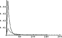
This simulates the output response of the closed-loop system to an impulse signal at the second input; in other words, it shows how the outflow rate and the concentration react to a short, sudden increase in the flow rate of the second chemical. The outflow rate and the concentration are shown as the dash-dotted and dotted lines, respectively.

In[8]:=

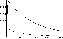
For comparison's sake, we plot the same graph for the original system. The outflow rate and the concentration are now shown as the solid and dashed lines.

In[9]:=

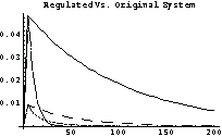
Finally, we combine the two plots in one graph, which shows clearly that the regulated system has a significantly faster response.

In[10]:=

A successful regulator design is possible only for a stabilizable system. Otherwise, LQRegulatorGains does not return any solution.

Here are matrices and for a system that is not stabilizable (because it is both unstable and uncontrollable).

In[11]:=

In[12]:=

We assign equal weight to all inputs and states.

In[13]:=

The attempt to build the regulator fails, as it should.

In[14]:=

Out[14]=

This modifies matrix so that the system is stable (though still uncontrollable).

In[15]:=

Now the regulator can be built.

In[16]:=

Out[16]=

The optimal regulator design is based on solving the appropriate algebraic Riccati equation. The corresponding functions—RiccatiSolve and DiscreteRiccatiSolve—can be accessed directly, if so desired, and are described in Section 10.3. LQRegulatorGains shares with the Riccati equation solvers the limitations imposed on the input arguments and accepts the options accepted by the Riccati solvers.